Top 18 How To Plot Stress Strain Curve In Abaqus 5992 Good Rating This Answer

You are looking for information, articles, knowledge about the topic nail salons open on sunday near me how to plot stress strain curve in abaqus on Google, you do not find the information you need! Here are the best content compiled and compiled by the https://chewathai27.com team, along with other related topics such as: how to plot stress strain curve in abaqus Stress strain curve abaqus, how to get stress strain curve in abaqus, abaqus plot force vs displacement, abaqus strain output, abaqus plot displacement vs time, Unit of strain in abaqus, how to apply strain in abaqus, strain in abaqus

Contents

How do you plot a strain stress curve?

The most common method for plotting a stress and strain curve is to subject a rod of the test piece to a tensile test. This is done using a Universal Testing Machine. It has two claws which hold the two extremes of the rod and pull it at a uniform rate.

How do you plot stress along a path in Abaqus?

Popular Answers (1)

Double-click on XYData on left.
Select ODB field output.
Select required stress measurement variable and select measurement location (unique nodal, element, etc.)
Select the desired nodes or elements from the field data (viewport) by clicking the Element/Nodes tab.
Save the Data.

How do you plot a graph on abaqus?

Select Tools XY Data Create from the main menu bar to launch the Create XY Data dialog box; then choose ODB history output. Click Continue. From the dialog box that appears, select one or more variables to plot and the step or steps of interest; then click Plot.

What is E in Abaqus?

For small-strain shells and beams in ABAQUS/Standard, the default strain measure, E, is Green’s strain: where is the deformation gradient and is the identity tensor. This strain measure is appropriate for the small-strain, large-rotation approximation used in these elements.

What is logarithmic strain?

The logarithmic strain provides the correct measure of the final strain when deformation takes place in a series of increments, taking into account the influence of the strain path.

How do you plot force displacement curve in Abaqus?

In the step module, specify the number of increments you want. Then, in the visualization module, go to Create XY data -> odb field output -> in the variables tab specify the variable(s) you want to plot and in the element/node tab specify the elements or nodes in which you want the results.

How do you plot deformation in Abaqus?

Click the contour icon , or select Plot > Contours > On Deformed Shape from the main toolbar. The default variable Abaqus/Viewer plots is the von Mises stress. Open the Field Output dialog box by selecting Result > Field Output to view state variables computed by Advanced Material Exchange.

How do you find the area under a stress-strain curve?

Using the starting length as L and the thickness and width you can calculate stress = load/area = N/mm2. Strain = deltaL/L (no units). The area under the curve is stress x strain. That gives the SI force unit of N/m2 which is pascals (Pa).

How do you convert a load deflection curve to a stress-strain curve?

To convert the load to stress, you divide the load by the area of the specimen tested. (i.e. N/mm2). Use the conversion factors to change this stress (N/mm2) to the units of your interest. For instance, converting the units to Pa, you can multiply the N/mm2 by a square of (1000mm/1m) which will give you N/m2.

How to get stress strain curve in ABAQUS

How to get stress strain curve in ABAQUS – YouTube

Article author: www.youtube.com
Reviews from users: 31418 Ratings
Top rated: 3.4
Lowest rated: 1
Summary of article content: Articles about How to get stress strain curve in ABAQUS – YouTube Updating …
Most searched keywords: Whether you are looking for How to get stress strain curve in ABAQUS – YouTube Updating #Abaqus #CAE_model #Hardening_cardDogbone model used in this video: https://drive.google.com/file/d/1HHoV8U9ipJbdJWsweNFVrNlbTdX9hGtT/view?usp=sharingGet for…video, chia sẻ, điện thoại có máy ảnh, điện thoại quay video, miễn phí, tải lên
Table of Contents:

Article author: fractory.com
Reviews from users: 41582 Ratings
Top rated: 4.8
Lowest rated: 1
Summary of article content: Articles about Stress-Strain Curve | How to Read the Graph? Updating …
Most searched keywords: Whether you are looking for Stress-Strain Curve | How to Read the Graph? Updating The stress-strain curve is one of the primary tools to assess a material’s properties. We’ll explain what insights you can get.
Table of Contents:

How to Read the Graph?

The stress-strain curve is one of the first material strength graphs we come across when starting on the journey to study materials.

While it is actually not that difficult, it may look a bit daunting at first. In this article, we shall learn about the stress and strain curve to understand it better.

But before we get there, we will try to explain a few key concepts for better comprehension.

Loading

A metal in service or during manufacturing is subjected to different forces. Depending on the magnitude of these forces, the metal may or may not change its shape.

The act of applying the force is known as loading. There are five different ways in which these forces may be applied on a metal part.

The five forms of loading are:

Compression Tension Shear Torsion Bending

Metals are elastic in nature up to a certain extent. When subjected to loading, the metal undergoes deformation but it may be too small to discern without special tools.

When this applied force is removed, the metal regains its original dimensions (unless the force exceeds a certain point). Just like a balloon, for example, regains its original shape after a force is removed after application.

What is Stress?

Stress is defined as the ratio of the applied force to the cross-sectional area of the material it is applied to.

The formula for calculating material stress:

σ=F/A, where

F is force (N)

A is area (m2)

σ is stress (N/m2 or Pa)

For example, a force of 1 N applied on a cross-sectional area of 1 m2, will be calculated as a stress of 1 N/m2 or 1 Pa. The unit can be both displayed as N/m2 or Pa, both of which represent pressure.

Stress can be understood as an internal force induced in the metal in response to an externally applied force. It will try to resist any change in dimension caused by the external force.

When the cross-sectional area changes, the same force will induce greater or smaller stresses in the metal. A smaller cross-sectional area will result in a larger stress value and vice versa.

What is Strain?

Strain is defined as the ratio of the change in dimension to the initial dimension of the metal. It does not have a unit.

There are three types of strain: normal, volumetric, and shear.

Normal strain (or longitudinal strain) concerns itself with the change in only one dimension, say length for example.

The formula for calculating strain is:

ε=(l-l 0 )/l 0 , where

l 0 is starting or initial length (mm)

l is stretched length (mm)

For example, if a certain force changes a metal’s length from 100 mm to 101 mm, the normal strain will be (101-100)/100 or 0.01.

Normal strain may be positive or negative depending on the external force’s directions and therefore effect on the original length.

For the sake of simplicity, we shall only talk about normal strain in our article. Thus, every time we use the word strain, it will refer to normal strain. Once we understand normal strain, it is easy to extend the same understanding to the other two.

Stress and Strain

Whenever a load acts on a body, it produces stress as well as strain in the material.

Let’s use a football as an example. When you try to squeeze it, it offers resistance. The resistance offered is the induced stress while the change in dimension represents the strain.

Strain causes stress. When applying force that leads to deformation, a material tries to retain its body structure by setting up internal stresses.

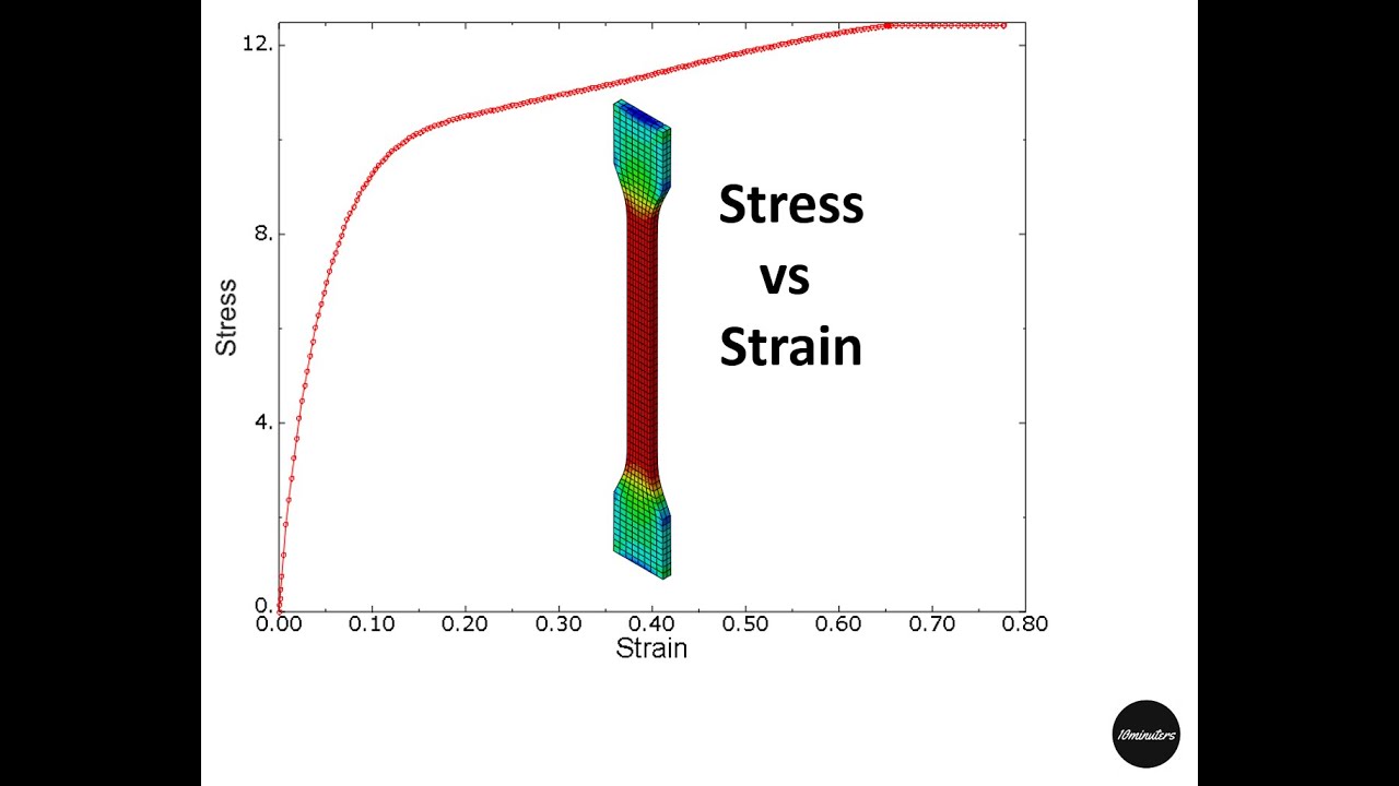
How is a Stress-Strain Curve Plotted?

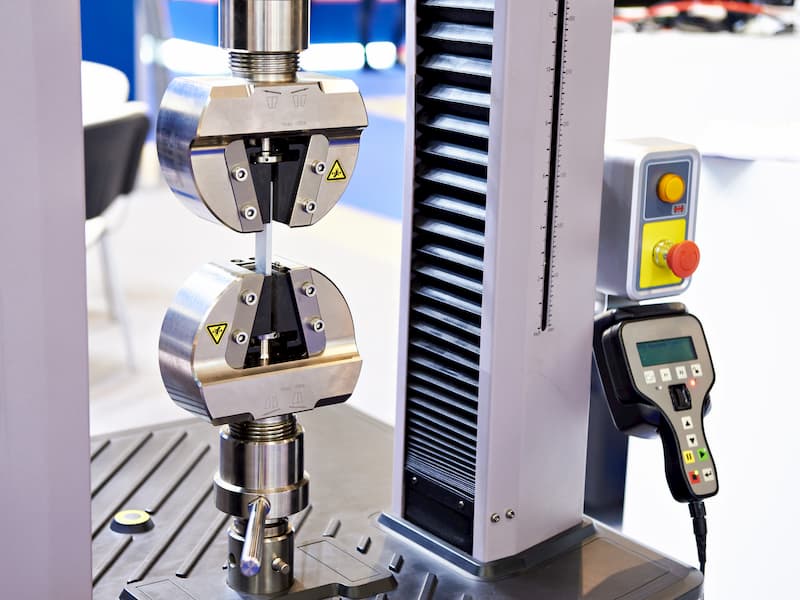
The most common method for plotting a stress and strain curve is to subject a rod of the test piece to a tensile test.

This is done using a Universal Testing Machine. It has two claws which hold the two extremes of the rod and pull it at a uniform rate.

The force applied and the strain produced is recorded until a fracture occurs. The two parameters are then plotted on an X-Y graph to get the familiar graph.

Stress-strain Curve

The stress-strain curve is a graph that shows the change in stress as strain increases. It is a widely used reference graph for metals in material science and manufacturing.

There are various sections on the stress and strain curve that describe different behaviour of a ductile material depending on the amount of stress induced.

Tensile test

Stress and strain curves for brittle, hard (but not ductile) and plastic materials are different. The curve for these materials is simpler and can be learned very easily. We shall focus on the stress-strain curve of ductile materials. But before we delve deeper into that, let’s take a look at another important concept – Hooke’s law.

Hooke’s Law

This principle of physics talks about elasticity and how the force required to extend or compress an elastic object by a certain distance is proportional to that distance. More force produces more distance.

Hooke’s law formula for calculating the force in springs:

In the case of metals, Hooke’s law dictates that for most metals, greater changes in length will create greater internal forces. That means stress is directly proportional to strain. This is because metals exhibit elasticity up to a certain limit.

In simple words, if the tensile/compressive load is doubled, the increase/decrease in length will also double as long as the metal is within the proportional limit.

Get your metal fabrication quote in seconds Quote in seconds

Short lead times

Delivery by Fractory Get quote

Proportional Limit

Almost all metals behave like an elastic object over a specific range. This range varies for different metals and is affected by factors such as mechanical properties, atmospheric exposure (corrosion), grain size, heat treatment, and working temperature.

When the testing machine starts pulling on the test piece, it undergoes tensile stress. Initially, the material follows Hooke’s law.

The strain will be proportional to stress. It means that the ratio of stress to strain will is a constant. In material science, this constant is known as Young’s modulus of elasticity and is one of the most important mechanical properties to consider when choosing the right material for an application.

There is no permanent deformation either. The metal will behave like a spring and return to its original dimension on the removal of load.

The point up to which this proportional behaviour is observed is known as the proportional limit. With increasing stress, strain increases linearly. In the diagram above, this rule applies up until the yields strength indicator.

Young’s Modulus of Elasticity

It is defined as the ratio of longitudinal stress to strain within the proportional limit of a material. Also known as modulus of resilience, it is analogous to the stiffness of a spring. That’s also why the Hooke’s law includes a spring constant.

Let’s say we have 2 materials with the same length and cross-section. To change the dimensions in equal measure, the material with a higher Young’s modulus value requires greater force.

Elastic Point & Yield Point

As the test piece is subjected to increasing amounts of tensile force, stresses increase beyond the proportional limit.

The stress-strain relationship deviates from Hooke’s law. The strain increases at a faster rate than stress which manifests itself as a mild flattening of the curve in the stress and strain graph.

This is the part of the graph where the first curve starts but has not yet taken a turn downwards. Although the proportionality of stress to strain is lost, the property of elasticity isn’t, and on the removal of load, the metal will still return to its original dimensions.

The change in dimension within the elastic limit is thus temporary and reversible. The elastic limit of a material ascertains its stability under stress.

Here lies the reason why engineering calculations use a material’s yield strength for determining its ability to resist a load. If the load is greater than the yield strength, the result will be unwanted plastic deformation.

Plastic Behaviour

When the test piece is pulled further on the testing machine, the property of elasticity is lost. This aligns with the start of the strain hardening region in the stress-strain graph.

The yield strength point is where the plastic deformation of the material is first observed. If the material is unclamped from the testing machine beyond this point, it will not return to its original length.

Strain hardening is said to occur when the number of dislocations in the material becomes too high and they start to obstruct each other’s movement. The material constantly rearranges itself and tends to harden.

Necking

The plastic deformation continues to occur with increasing stress. In due time, a narrowing of cross-section will be observed at a point on the rod. This phenomenon is known as necking. The stress is so high that it leads to the formation of a neck at the weakest point of the rod. You can see this happen in the video above.

The stress-strain curve also shown the region where necking occurs. Its starting-point also gives us the ultimate tensile strength of a material.

Ultimate tensile strength shows the maximum amount of stress a material can handle. Reaching this value pushes the material towards failure and breaking.

Fracture

Once in the necking region, we can see that the load does not have to increase for further plastic deformation.

A fracture will occur at the neck usually with a cup and cone shape formation at either end of the rod. This point is known as the fracture or rupture point and is denoted by E on the stress and strain graph.

Why is the Strain-Stress Curve Important?

The stress-strain curve provides design engineers with a long list of important parameters needed for application design. A stress-strain graph gives us many mechanical properties such as strength, toughness, elasticity, yield point, strain energy, resilience, and elongation during load.

It also helps in fabrication. Whether you are looking to perform extrusion, rolling, bending or some other operation, the values stemming from this graph will help you to determine the forces necessary to induce plastic deformation.

47.3 Producing an X–Y plot

X–Y plot

47.3 Producing anplot

To produce an X–Y plot, you first specify an X–Y data object. You can then choose to simply plot the specified X–Y data object or to save the data object and plot it later.

History and field data objects can include complex numbers; you can control the displayed form of complex numbers using the Result Options dialog box. An abbreviation of the complex form is appended to the Y-axis title when you plot the variable and becomes part of the saved variable name. For example, if S-Mises is the selected field output variable and Magnitude is the complex form, the Y-axis title is S-Mises CPX: Mg . For more information on complex number forms in Abaqus/CAE, see “Controlling the form of complex results,” Section 42.6.9.

Use one of the following methods to produce an X–Y plot:

To produce an X–Y plot of history data from an output database: Select Tools XY Data Create from the main menu bar to launch the Create XY Data dialog box; then choose ODB history output. Click Continue. From the dialog box that appears, select one or more variables to plot and the step or steps of interest; then click Plot. Tip: To launch the Create XY Data dialog box from the Results Tree, click mouse button 3 on the XYData container and select Create from the list that appears. You can also specify history output by selecting Result History Output from the main menu bar.

To produce an X–Y plot of field data from an output database: Select Tools XY Data Create from the main menu bar; then choose ODB field output. Click Continue. From the dialog box that appears, select one or more variables to plot, the location or locations from which to read the data, and the step or steps of interest; then click Plot.

To produce an X–Y plot of output database results along a path through your model: To specify a path through your model, select Tools Path Create from the main menu bar; then configure the dialog boxes that appear. For more information, see “Creating a path through your model,” Section 48.2. After you have created the path, select Tools XY Data Create from the main menu bar. Choose Path as the source of the X–Y data object, then click Continue. Configure the dialog box that appears, then click Plot. For more information, see “Obtaining X–Y data along a path,” Section 48.3.

To produce an X–Y plot of new data, not from an output database: Select Tools XY Data Create from the main menu bar. Choose either Operate on XY data, ASCII file, or Keyboard as the source of the X–Y data object; then click Continue. In the dialog box that appears, enter your X–Y data object; then click Plot (or Plot Expression in the Operate on XY Data dialog box).

To produce an X–Y plot of one or more saved X–Y data objects: To display a single X–Y data object, select Tools XY Data Plot from the main menu bar; and select the X–Y data object from the pull-right menu.

To display multiple X–Y data objects on a single X–Y plot, select Tools XY Data Manager from the main menu bar. Select the X–Y data objects from the dialog box that appears; then click Plot. You can also perform either of these actions from the Results Tree. To display a single X–Y data object using the Results Tree, expand the XYData container, click mouse button 3 on the X–Y data object you want to plot, and select Plot from the list that appears. To display multiple X–Y data objects using the Results Tree, highlight multiple X–Y objects under the XYData container, click mouse button 3 on one of the highlighted objects, and select Plot from the list that appears.

For information on related topics, click any of the following items:

10.2 Plasticity in ductile metals

Many metals have approximately linear elastic behavior at low strain magnitudes (see Figure 101 ), and the stiffness of the material, known as the Young’s or elastic modulus, is constant.

10.2.1 Characteristics of plasticity in ductile metals

The plastic behavior of a material is described by its yield point and its post-yield hardening. The shift from elastic to plastic behavior occurs at a certain point, known as the elastic limit or yield point, on a material’s stress-strain curve (see Figure 102). The stress at the yield point is called the yield stress. In most metals the initial yield stress is 0.05 to 0.1% of the material’s elastic modulus.

The deformation of the metal prior to reaching the yield point creates only elastic strains, which are fully recovered if the applied load is removed. However, once the stress in the metal exceeds the yield stress, permanent (plastic) deformation begins to occur. The strains associated with this permanent deformation are called plastic strains. Both elastic and plastic strains accumulate as the metal deforms in the post-yield region.

The stiffness of a metal typically decreases dramatically once the material yields (see Figure 102). A ductile metal that has yielded will recover its initial elastic stiffness when the applied load is removed (see Figure 102). Often the plastic deformation of the material increases its yield stress for subsequent loadings: this behavior is called work hardening.

Another important feature of metal plasticity is that the inelastic deformation is associated with nearly incompressible material behavior. Modeling this effect places some severe restrictions on the type of elements that can be used in elastic-plastic simulations.

A metal deforming plastically under a tensile load may experience highly localized extension and thinning, called necking, as the material fails (see Figure 102). The engineering stress (force per unit undeformed area) in the metal is known as the nominal stress, with the conjugate nominal strain (length change per unit undeformed length). The nominal stress in the metal as it is necking is much lower than the material’s ultimate strength. This material behavior is caused by the geometry of the test specimen, the nature of the test itself, and the stress and strain measures used. For example, testing the same material in compression produces a stress-strain plot that does not have a necking region because the specimen is not going to thin as it deforms under compressive loads. A mathematical model describing the plastic behavior of metals should be able to account for differences in the compressive and tensile behavior independent of the structure’s geometry or the nature of the applied loads. This goal can be accomplished if the familiar definitions of nominal stress, , and nominal strain, , where the subscript 0 indicates a value from the undeformed state of the material, are replaced by new measures of stress and strain that account for the change in area during the finite deformations.

So you have finished reading the how to plot stress strain curve in abaqus topic article, if you find this article useful, please share it. Thank you very much. See more: Stress strain curve abaqus, how to get stress strain curve in abaqus, abaqus plot force vs displacement, abaqus strain output, abaqus plot displacement vs time, Unit of strain in abaqus, how to apply strain in abaqus, strain in abaqus

Top 18 How To Plot Stress Strain Curve In Abaqus 5992 Good Rating This Answer

How do you plot a strain stress curve?

How do you plot stress along a path in Abaqus?

How do you plot a graph on abaqus?

What is E in Abaqus?

What is logarithmic strain?

How do you plot force displacement curve in Abaqus?

How do you plot deformation in Abaqus?

How do you find the area under a stress-strain curve?

How do you convert a load deflection curve to a stress-strain curve?

How to get stress strain curve in ABAQUS – YouTube

Stress-Strain Curve | How to Read the Graph?

47.3 Producing an X–Y plot

10.2 Plasticity in ductile metals

Plotting stress-strain graph from simulation | iMechanica

how to plot stress strain curve in abaqus

Error 403 (Forbidden)

How to Read the Graph?

47.3 Producing an X–Y plot

10.2 Plasticity in ductile metals

Leave a Comment Cancel reply