Top 27 How To Get Histogram On Ti 84 Plus 455 People Liked This Answer

You are looking for information, articles, knowledge about the topic nail salons open on sunday near me how to get histogram on ti 84 plus on Google, you do not find the information you need! Here are the best content compiled and compiled by the Chewathai27.com team, along with other related topics such as: how to get histogram on ti 84 plus how to graph histogram on calculator, how to change bin width on ti-84, how to make a boxplot on ti-84, how to make a relative frequency histogram on a ti-84, how to make a histogram, ti-84 histogram invalid dim, histogram graphing calculator, frequency distribution ti-84

Contents

How do you graph a relative frequency histogram on a TI 84?

TI-84: Histograms

Turn your Stat Plot ON and select the Histogram Icon. …
Go to STAT –> Edit. …
Type values into L1. …
Go to Zoom Stat (Zoom 9) to view and to create a friendly window. …
Use the TRACE button and arrow keys to toggle through the bars of the histogram.

How do you plot a histogram?

Making a Histogram Using a Frequency Distribution Table

On the vertical axis, place frequencies. Label this axis “Frequency”.
On the horizontal axis, place the lower value of each interval. …
Draw a bar extending from the lower value of each interval to the lower value of the next interval.

How do you graph stats on a TI 84?

TI-84: Setting Up a Scatter Plot

Go to [2nd] “STAT PLOT”. Make sure that only Plot1 is ON. …
Go to Y1 and [Clear] any functions.
Go to [STAT] [EDIT]. Enter your data in L1 and L2.
Then go to [ZOOM] “9: ZoomStat” to see the scatter plot in a “friendly window”.
Press [TRACE] and the arrow keys to view each data point.

How do you reset a TI 84 Plus calculator?

Q: How can I completely reset my TI 84 Plus back to the factory default settings?

Press 2nd MEM (that is the second function of the + key)
Choose 7 (Reset)
Scroll right so that ALL is selected.
Press 1.
Press 2 (Reset, and read the warnings)

What is a frequency histogram?

A histogram or frequency histogram consists of a set of rectangles having: (1) bases on a horizontal axis (the x-axis) with centers at the class midpoint and lengths equal to the class interval sizes; (2) areas that are proportional to class frequencies.

Is histogram and bar graph the same?

A bar graph is the graphical representation of categorical data using rectangular bars where the length of each bar is proportional to the value they represent. A histogram is the graphical representation of data where data is grouped into continuous number ranges and each range corresponds to a vertical bar.

How do you draw a histogram for grouped data?

HOW TO DRAW HISTOGRAM FOR GROUPED DATA

Step 1 : Represent the data in the continuous (exclusive) form if it is in the discontinuous (inclusive) form.
Step 2 : Mark the class intervals along the X-axis on a uniform scale.
Step 3 : Mark the frequencies along the Y-axis on a uniform scale.
Step 4 :

How do you make a Boxplot on TI 84?

TI-84: Box Plots

Turn on the Stat Plot. Press [2nd] [Stat Plot]. …
Select a Box Plot icon. The first one will show outliers. …
Enter Data in L1 of [Stat]
View Box Plot by going to [ZOOM] ‘Stat’ (#9). …
Press [Trace] and the arrow keys to view the values of the Min, Q1, Median, Q3, and Max.
Go to the [2nd] [Stat].

What is a frequency histogram?

Statistics – How to make a histogram using the TI-83/84 calculator

TI-84: Histograms | TI-84 Graphing Calculator | CPM Student Tutorials

Article author: studenthelp.cpm.org
Reviews from users: 44431 Ratings
Top rated: 5.0
Lowest rated: 1
Summary of article content: Articles about TI-84: Histograms | TI-84 Graphing Calculator | CPM Student Tutorials 1. Turn your Stat Plot ON and select the Histogram Icon. … Select [2nd[ [Stat Plot]. Use the arrow keys to turn the Stat Plot “On”. Press ‘ENTER … …
Most searched keywords: Whether you are looking for TI-84: Histograms | TI-84 Graphing Calculator | CPM Student Tutorials 1. Turn your Stat Plot ON and select the Histogram Icon. … Select [2nd[ [Stat Plot]. Use the arrow keys to turn the Stat Plot “On”. Press ‘ENTER …
Table of Contents:

Watch the 3 minute video or follow the steps below it

1 Turn your Stat Plot ON and select the Histogram Icon

2 Go to STAT — Edit Press ‘ENTER’

3 Type values into L1 Press ‘ENTER’ after each entry

4 Go to Zoom Stat (Zoom 9) to view and to create a friendly window

5 Use the TRACE button and arrow keys to toggle through the bars of the histogram

6 Change the bin by going into Window and changing the x scale

7 Press GRAPH The new histogram will reflect new heights of the bars with a different bin value

TI-84: Histograms | TI-84 Graphing Calculator | CPM Student Tutorials

Article author: www.youtube.com
Reviews from users: 12314 Ratings
Top rated: 4.3
Lowest rated: 1
Summary of article content: Articles about Making Histograms with a TI-84 Plus & Manually Adjusting Classes – YouTube Updating …
Most searched keywords: Whether you are looking for Making Histograms with a TI-84 Plus & Manually Adjusting Classes – YouTube Updating This video demonstration shows how to make a histogram with a TI-84, TI-84 Plus, TI-83, or TI-83 Plus. This video also show how to manually adjust the classe…ap statistics, histogram, TI-84, TI-84 Plus, TI-83, TI-83 Plus, manually adjusting classes, class, range, scale
Table of Contents:

Making Histograms with a TI-84 Plus & Manually Adjusting Classes - YouTube — Making Histograms with a TI-84 Plus & Manually Adjusting Classes – YouTube

Article author: www.youtube.com
Reviews from users: 10898 Ratings
Top rated: 4.5
Lowest rated: 1
Summary of article content: Articles about Statistics – How to make a histogram using the TI-83/84 calculator – YouTube Updating …
Most searched keywords: Whether you are looking for Statistics – How to make a histogram using the TI-83/84 calculator – YouTube Updating This video shows how to make a histogram using the TI-83 or TI-84 calculator. Remember to set your window and plot options before graphing the data. For mo…Statistics, Histogram, Make, Graph, Plot, TI-83, TI-84, Graphing, Calculator
Table of Contents:

Statistics - How to make a histogram using the TI-83/84 calculator - YouTube — Statistics – How to make a histogram using the TI-83/84 calculator – YouTube

Article author: studenthelp.cpm.org
Reviews from users: 12138 Ratings
Top rated: 3.3
Lowest rated: 1
Summary of article content: Articles about TI-84: Histograms | TI-84 Graphing Calculator | CPM Student Tutorials Updating …
Most searched keywords: Whether you are looking for TI-84: Histograms | TI-84 Graphing Calculator | CPM Student Tutorials Updating
Table of Contents:

Watch the 3 minute video or follow the steps below it

1 Turn your Stat Plot ON and select the Histogram Icon

2 Go to STAT — Edit Press ‘ENTER’

3 Type values into L1 Press ‘ENTER’ after each entry

4 Go to Zoom Stat (Zoom 9) to view and to create a friendly window

5 Use the TRACE button and arrow keys to toggle through the bars of the histogram

6 Change the bin by going into Window and changing the x scale

7 Press GRAPH The new histogram will reflect new heights of the bars with a different bin value

TI-84: Histograms | TI-84 Graphing Calculator | CPM Student Tutorials

Article author: www.sparknotes.com
Reviews from users: 10710 Ratings
Top rated: 4.4
Lowest rated: 1
Summary of article content: Articles about Graphing Data: Histograms | SparkNotes Updating …
Most searched keywords: Whether you are looking for Graphing Data: Histograms | SparkNotes Updating Graphing Data quizzes about important details and events in every section of the book.Graphing Data, Histograms, , scene summary, scene summaries, chapter summary, chapter summaries, short summary, criticism, literary criticism, review, scene synopsis, interpretation, teaching, lesson plan
Table of Contents:

Reset Password

Math

Unlock your FREE SparkNotes PLUS trial!

Unlock your FREE Trial!

Histograms

SparkNotes—the stress-free way to a better GPA

Article author: www.dummies.com
Reviews from users: 30843 Ratings
Top rated: 4.5
Lowest rated: 1
Summary of article content: Articles about How to Construct Histograms on the TI-84 Plus Article – dummies Press the down-arrow key, use the right-arrow key to place the cursor on the type of plot you want to create, and then press e to highlight it. …
Most searched keywords: Whether you are looking for How to Construct Histograms on the TI-84 Plus Article – dummies Press the down-arrow key, use the right-arrow key to place the cursor on the type of plot you want to create, and then press e to highlight it. The most common plots used to graph one-variable data are histograms and box plots. In a histogram, the data is grouped into classes of equal size; a bar in the
Table of Contents:

Article Categories

Book Categories

Collections

Adjusting the class size of a histogram

About This Article

How to Construct Histograms on the TI-84 Plus Article – dummies

Article author: www.mathbootcamps.com
Reviews from users: 48800 Ratings
Top rated: 4.3
Lowest rated: 1
Summary of article content: Articles about Histograms with a Graphing Calculator The TI83 and TI84 graphing calculators give us a nice and easy way to get a histogram in order to see the overall pattern of a data set (which is the goal … …
Most searched keywords: Whether you are looking for Histograms with a Graphing Calculator The TI83 and TI84 graphing calculators give us a nice and easy way to get a histogram in order to see the overall pattern of a data set (which is the goal … The basic steps to getting and reading a histogram from a TI83 or 84 calculator using a small example.
Table of Contents:

Example (video example)

Video Example

What if there is an error

Graphing Data: Histograms

Frequency Distribution Tables

A frequency distribution table is a table that shows how often a data point or a group of data points appears in a given data set. To make a frequency distribution table, first divide the numbers over which the data ranges into intervals of equal length. Then count how many data points fall into each interval.

If there are many values, it is sometimes useful to go through all the data points in order and make a tally mark in the interval that each point falls. Then all the tally marks can be counted to see how many data points fall into each interval. The “tally system” ensures that no points will be missed.

Example: The following is a list of prices (in dollars) of birthday cards found in various drug stores:

1.45 2.20 0.75 1.23 1.25 1.25 3.09 1.99 2.00 0.78 1.32 2.25 3.15 3.85 0.52 0.99 1.38 1.75 1.22 1.75

0.52

3.85

0.50

4.00

7

0.50 – 0.99

1.00 – 1.49

1.50 – 1.99

2.00 – 2.49

2.50 – 2.99

3.00 – 3.49

3.50 – 3.99

Intervals (in dollars) Frequency 0.50 – 0.99 4 1.00 – 1.49 7 1.50 – 1.99 3 2.00 – 2.49 3 2.50 – 2.99 3.00 – 3.49 2 3.50 – 3.99 1 Total 20

Making a Histogram Using a Frequency Distribution Table

Make a frequency distribution table for this data.

A histogram is a bar graph which shows frequency distribution.

To make a histogram, follow these steps:

On the vertical axis, place frequencies. Label this axis “Frequency”. On the horizontal axis, place the lower value of each interval. Label this axis with the type of data shown (price of birthday cards, etc.) Draw a bar extending from the lower value of each interval to the lower value of the next interval. The height of each bar should be equal to the frequency of its corresponding interval.

Histogram

Information From a Histogram

: Make a histogram showing the frequency distribution of the price of birthday cards.

Histograms are useful because they allow us to glean certain information at a glance. The previous example shows that more birthday cards cost between $1.00 and $1.49 than any other price, because the bar which corresponds to those values is highest. We can also see that twice as many cards cost between $3.00 – $3.49 as cost between $3.50 – $3.99, because the bar which corresponds to $3.00 – $3.49 is twice as high as the bar which corresponds to $3.50 – $3.99.

How to Construct Histograms on the TI-84 Plus Article

{“appState”:{“pageLoadApiCallsStatus”:true},”articleState”:{“article”:{“headers”:{“creationTime”:”2016-03-26T14:01:48+00:00″,”modifiedTime”:”2016-03-26T14:01:48+00:00″,”timestamp”:”2022-06-22T19:22:07+00:00″},”data”:{“breadcrumbs”:[{“name”:”Technology”,”_links”:{“self”:”https://dummies-api.dummies.com/v2/categories/33512″},”slug”:”technology”,”categoryId”:33512},{“name”:”Electronics”,”_links”:{“self”:”https://dummies-api.dummies.com/v2/categories/33543″},”slug”:”electronics”,”categoryId”:33543},{“name”:”Graphing Calculators”,”_links”:{“self”:”https://dummies-api.dummies.com/v2/categories/33551″},”slug”:”graphing-calculators”,”categoryId”:33551}],”title”:”How to Construct Histograms on the TI-84 Plus”,”strippedTitle”:”how to construct histograms on the ti-84 plus”,”slug”:”how-to-construct-histograms-on-the-ti-84-plus”,”canonicalUrl”:””,”seo”:{“metaDescription”:”The most common plots used to graph one-variable data are histograms and box plots. In a histogram, the data is grouped into classes of equal size; a bar in the”,”noIndex”:0,”noFollow”:0},”content”:”

The most common plots used to graph one-variable data are histograms and box plots. In a histogram, the data is grouped into classes of equal size; a bar in the histogram represents one class. The height of the bar represents the quantity of data contained in that class. To construct a histogram of your data on your TI-84 Plus, follow these steps:

Enter your data in the calculator.

See the first screen. Your list does not have to appear in the Stat List editor to plot it, but it does have to be in the memory of the calculator.

$\"image0.jpg\"/$

Turn off any Stat Plots or functions in the Y= editor that you don’t want to be graphed along with your histogram.

To do so, press [Y=] to access the Y= editor. The calculator graphs any highlighted plots in the first line of this editor. To remove the highlight from a plot so that it won’t be graphed, use the arrow keys to place the cursor on the plot and then press [ENTER] to toggle the plot between highlighted and not highlighted.

The calculator graphs only those functions in the Y= editor defined by a highlighted equal sign. To remove the highlight from an equal sign, use the arrow keys to place the cursor on the equal sign in the definition of the function, and then press [ENTER] to toggle the equal sign between highlighted and not highlighted. See the second screen.

Press [2nd][Y=] to access the Stat Plots menu and enter the number (1, 2, or 3) of the plot you want to define.

The third screen shows this process, where Plot1 is used to plot the data.

Highlight On.

If On is highlighted, the calculator is set to plot your data. If you want your data to be plotted at a later time, highlight Off. To highlight an option, use the arrow keys to place the cursor on the option, and then press [ENTER].

Press the down-arrow key, use the right-arrow key to place the cursor on the type of plot you want to create, and then press e to highlight it.

Select the icon that looks like a city skyline (or cell phone bars) to construct a histogram.

Press the down-arrow key, enter the name of your data list (Xlist), and press [ENTER].

If your data is stored in one of the default lists L₁ through L₆, press [2nd], key in the number of the list, and then press [ENTER]. For example, press [2nd][1] if your data is stored in L₁.

If your data is stored in a user-named list, key in the name of the list and press [ENTER] when you’re finished.

You can always access a list by pressing [2nd][STAT] and using the up- and down-arrow keys to scroll through all the stored lists in your calculator.

Enter the frequency of your data.

If you entered your data without paying attention to duplicate data values, then the frequency is 1. On the other hand, if you did pay attention to duplicate data values, you most likely stored the frequency in another data list. If so, enter the name of that list the same way you entered the Xlist in Step 6.

Choose the color of your histogram.

Use the left- and right-arrow keys to operate the menu spinner to choose one of 15 color options. See the first screen.

$\"image1.jpg\"/$

Press [ZOOM][9] to plot your data using the ZoomStat command.

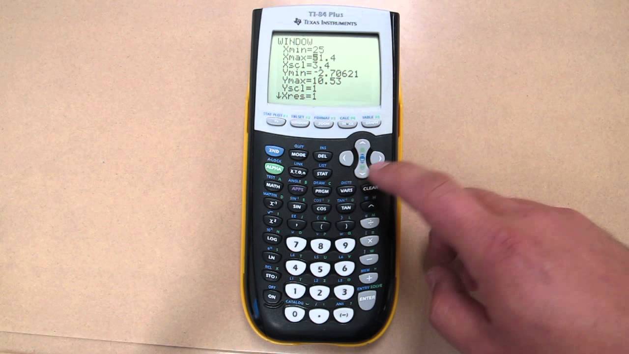
ZoomStat finds an appropriate viewing window for plotting your data, as shown in the second screen. If you are not pleased with the graphing window that is generated, press [WINDOW] and change your values manually.

Adjusting the class size of a histogram

When creating a histogram, your calculator groups data into \”classes.\” The data in the first screen has been split into six classes represented by the six bars in the histogram.

$\"image2.jpg\"/$

The class size (also called the class interval) is the width of each bar in the histogram. If you have more than 46 classes, your calculator will return the ERROR: STAT error message. Here is a formula that can be used to compute the class size:

Class size = (max – min)/(number of classes you want to have)

To adjust the class size of a histogram, follow these steps:

Press [WINDOW], set Xscl equal to the class size you desire, and then press [GRAPH].

To change the class size, change the value of Xscl in your calculator. See the graph after changing the Xscl in the second screen.

If necessary, adjust the settings in the Window editor.

When the histogram is graphed again using a different class size (as shown in the second screen), the viewing window doesn’t do a good job of accommodating the histogram. To correct this, adjust the settings in the Window editor. The Ymax settings were changed to produce the third screen.

“,”description”:”

The most common plots used to graph one-variable data are histograms and box plots. In a histogram, the data is grouped into classes of equal size; a bar in the histogram represents one class. The height of the bar represents the quantity of data contained in that class. To construct a histogram of your data on your TI-84 Plus, follow these steps:

Enter your data in the calculator.

See the first screen. Your list does not have to appear in the Stat List editor to plot it, but it does have to be in the memory of the calculator.

$\"image0.jpg\"/$

Turn off any Stat Plots or functions in the Y= editor that you don’t want to be graphed along with your histogram.

To do so, press [Y=] to access the Y= editor. The calculator graphs any highlighted plots in the first line of this editor. To remove the highlight from a plot so that it won’t be graphed, use the arrow keys to place the cursor on the plot and then press [ENTER] to toggle the plot between highlighted and not highlighted.

The calculator graphs only those functions in the Y= editor defined by a highlighted equal sign. To remove the highlight from an equal sign, use the arrow keys to place the cursor on the equal sign in the definition of the function, and then press [ENTER] to toggle the equal sign between highlighted and not highlighted. See the second screen.

Press [2nd][Y=] to access the Stat Plots menu and enter the number (1, 2, or 3) of the plot you want to define.

The third screen shows this process, where Plot1 is used to plot the data.

Highlight On.

If On is highlighted, the calculator is set to plot your data. If you want your data to be plotted at a later time, highlight Off. To highlight an option, use the arrow keys to place the cursor on the option, and then press [ENTER].

Press the down-arrow key, use the right-arrow key to place the cursor on the type of plot you want to create, and then press e to highlight it.

Select the icon that looks like a city skyline (or cell phone bars) to construct a histogram.

Press the down-arrow key, enter the name of your data list (Xlist), and press [ENTER].

If your data is stored in one of the default lists L₁ through L₆, press [2nd], key in the number of the list, and then press [ENTER]. For example, press [2nd][1] if your data is stored in L₁.

If your data is stored in a user-named list, key in the name of the list and press [ENTER] when you’re finished.

You can always access a list by pressing [2nd][STAT] and using the up- and down-arrow keys to scroll through all the stored lists in your calculator.

Enter the frequency of your data.

If you entered your data without paying attention to duplicate data values, then the frequency is 1. On the other hand, if you did pay attention to duplicate data values, you most likely stored the frequency in another data list. If so, enter the name of that list the same way you entered the Xlist in Step 6.

Choose the color of your histogram.

Use the left- and right-arrow keys to operate the menu spinner to choose one of 15 color options. See the first screen.

$\"image1.jpg\"/$

Press [ZOOM][9] to plot your data using the ZoomStat command.

ZoomStat finds an appropriate viewing window for plotting your data, as shown in the second screen. If you are not pleased with the graphing window that is generated, press [WINDOW] and change your values manually.

Adjusting the class size of a histogram

When creating a histogram, your calculator groups data into \”classes.\” The data in the first screen has been split into six classes represented by the six bars in the histogram.

$\"image2.jpg\"/$

The class size (also called the class interval) is the width of each bar in the histogram. If you have more than 46 classes, your calculator will return the ERROR: STAT error message. Here is a formula that can be used to compute the class size:

Class size = (max – min)/(number of classes you want to have)

To adjust the class size of a histogram, follow these steps:

Press [WINDOW], set Xscl equal to the class size you desire, and then press [GRAPH].

To change the class size, change the value of Xscl in your calculator. See the graph after changing the Xscl in the second screen.

If necessary, adjust the settings in the Window editor.

When the histogram is graphed again using a different class size (as shown in the second screen), the viewing window doesn’t do a good job of accommodating the histogram. To correct this, adjust the settings in the Window editor. The Ymax settings were changed to produce the third screen.

“,”blurb”:””,”authors”:[{“authorId”:9554,”name”:”Jeff McCalla”,”slug”:”jeff-mccalla”,”description”:”

Jeff McCalla teaches Algebra 2 and Pre-Calculus at St. Mary’s Episcopal School in Memphis. He is a T3 instructor for Texas Instruments and co- founder of the TI-Nspire SuperUser group.

Steve Ouellette wrote the first edition of TI-Nspire For Dummies as well as CliffsNotes^® Guide to TI-Nspire.

“,”_links”:{“self”:”https://dummies-api.dummies.com/v2/authors/9554″}},{“authorId”:9555,”name”:”C. C. Edwards”,”slug”:”c-c-edwards”,”description”:”C.C. Edwards is a teacher and a former editor of Texas Instruments’ Eightysomething, a newsletter for parents and educators.”,”_links”:{“self”:”https://dummies-api.dummies.com/v2/authors/9555″}}],”primaryCategoryTaxonomy”:{“categoryId”:33551,”title”:”Graphing Calculators”,”slug”:”graphing-calculators”,”_links”:{“self”:”https://dummies-api.dummies.com/v2/categories/33551″}},”secondaryCategoryTaxonomy”:{“categoryId”:0,”title”:null,”slug”:null,”_links”:null},”tertiaryCategoryTaxonomy”:{“categoryId”:0,”title”:null,”slug”:null,”_links”:null},”trendingArticles”:null,”inThisArticle”:[{“label”:”Adjusting the class size of a histogram”,”target”:”#tab1″}],”relatedArticles”:{“fromBook”:[{“articleId”:257053,”title”:”How to Find Standard Deviation on the TI-84 Graphing Calculator”,”slug”:”how-to-find-standard-deviation-on-the-ti-84-graphing-calculator”,”categoryList”:[“technology”,”electronics”,”graphing-calculators”],”_links”:{“self”:”https://dummies-api.dummies.com/v2/articles/257053″}},{“articleId”:209964,”title”:”How to Enable and Disable the TI-TestGuard App on a Class Set of TI-84 Plus Calculators”,”slug”:”how-to-enable-and-disable-the-ti-testguard-app-on-a-class-set-of-ti-84-plus-calculators”,”categoryList”:[“technology”,”electronics”,”graphing-calculators”],”_links”:{“self”:”https://dummies-api.dummies.com/v2/articles/209964″}},{“articleId”:209962,”title”:”How to Store a Picture on the TI-84 Plus”,”slug”:”how-to-store-a-picture-on-the-ti-84-plus”,”categoryList”:[“technology”,”electronics”,”graphing-calculators”],”_links”:{“self”:”https://dummies-api.dummies.com/v2/articles/209962″}},{“articleId”:209963,”title”:”How to Download and Install the TI-TestGuard App on the TI-84 Plus”,”slug”:”how-to-download-and-install-the-ti-testguard-app-on-the-ti-84-plus”,”categoryList”:[“technology”,”electronics”,”graphing-calculators”],”_links”:{“self”:”https://dummies-api.dummies.com/v2/articles/209963″}},{“articleId”:207962,”title”:”TI-84 Plus C Graphing Calculator For Dummies Cheat Sheet”,”slug”:”ti-84-plus-graphing-calculator-for-dummies-cheat-sheet”,”categoryList”:[“technology”,”electronics”,”graphing-calculators”],”_links”:{“self”:”https://dummies-api.dummies.com/v2/articles/207962″}}],”fromCategory”:[{“articleId”:257053,”title”:”How to Find Standard Deviation on the TI-84 Graphing Calculator”,”slug”:”how-to-find-standard-deviation-on-the-ti-84-graphing-calculator”,”categoryList”:[“technology”,”electronics”,”graphing-calculators”],”_links”:{“self”:”https://dummies-api.dummies.com/v2/articles/257053″}},{“articleId”:209964,”title”:”How to Enable and Disable the TI-TestGuard App on a Class Set of TI-84 Plus Calculators”,”slug”:”how-to-enable-and-disable-the-ti-testguard-app-on-a-class-set-of-ti-84-plus-calculators”,”categoryList”:[“technology”,”electronics”,”graphing-calculators”],”_links”:{“self”:”https://dummies-api.dummies.com/v2/articles/209964″}},{“articleId”:209962,”title”:”How to Store a Picture on the TI-84 Plus”,”slug”:”how-to-store-a-picture-on-the-ti-84-plus”,”categoryList”:[“technology”,”electronics”,”graphing-calculators”],”_links”:{“self”:”https://dummies-api.dummies.com/v2/articles/209962″}},{“articleId”:209963,”title”:”How to Download and Install the TI-TestGuard App on the TI-84 Plus”,”slug”:”how-to-download-and-install-the-ti-testguard-app-on-the-ti-84-plus”,”categoryList”:[“technology”,”electronics”,”graphing-calculators”],”_links”:{“self”:”https://dummies-api.dummies.com/v2/articles/209963″}},{“articleId”:209198,”title”:”TI-89 Graphing Calculator For Dummies Cheat Sheet”,”slug”:”ti-89-graphing-calculator-for-dummies-cheat-sheet”,”categoryList”:[“technology”,”electronics”,”graphing-calculators”],”_links”:{“self”:”https://dummies-api.dummies.com/v2/articles/209198″}}]},”hasRelatedBookFromSearch”:false,”relatedBook”:{“bookId”:281880,”slug”:”ti-84-plus-graphing-calculator-for-dummies-2nd-edition”,”isbn”:”9781118592151″,”categoryList”:[“technology”,”electronics”,”graphing-calculators”],”amazon”:{“default”:”https://www.amazon.com/gp/product/1118592158/ref=as_li_tl?ie=UTF8&tag=wiley01-20″,”ca”:”https://www.amazon.ca/gp/product/1118592158/ref=as_li_tl?ie=UTF8&tag=wiley01-20″,”indigo_ca”:”http://www.tkqlhce.com/click-9208661-13710633?url=https://www.chapters.indigo.ca/en-ca/books/product/1118592158-item.html&cjsku=978111945484″,”gb”:”https://www.amazon.co.uk/gp/product/1118592158/ref=as_li_tl?ie=UTF8&tag=wiley01-20″,”de”:”https://www.amazon.de/gp/product/1118592158/ref=as_li_tl?ie=UTF8&tag=wiley01-20″},”image”:{“src”:”https://www.dummies.com/wp-content/uploads/ti-84-plus-graphing-calculator-for-dummies-2nd-edition-cover-9781118592151-202×255.jpg”,”width”:202,”height”:255},”title”:”Ti-84 Plus Graphing Calculator For Dummies”,”testBankPinActivationLink”:””,”bookOutOfPrint”:false,”authorsInfo”:”

Jeff McCalla is a mathematics teacher at St. Mary’s Episcopal School in Memphis, TN. He cofounded the TI-Nspire SuperUser group, and received the Presidential Award for Excellence in Science & Mathematics Teaching. C.C. Edwards is an educator who has presented numerous workshops on using TI calculators.

“,”authors”:[{“authorId”:9554,”name”:”Jeff McCalla”,”slug”:”jeff-mccalla”,”description”:”

Jeff McCalla teaches Algebra 2 and Pre-Calculus at St. Mary’s Episcopal School in Memphis. He is a T3 instructor for Texas Instruments and co- founder of the TI-Nspire SuperUser group.

Steve Ouellette wrote the first edition of TI-Nspire For Dummies as well as CliffsNotes^® Guide to TI-Nspire.

“,”_links”:{“self”:”https://dummies-api.dummies.com/v2/authors/9554″}},{“authorId”:34843,”name”:”C. C. Edwards”,”slug”:”c.-c.-edwards”,”description”:”

C.C. Edwards is an instructor at Coastal Carolina University and a former editor of Texas Instruments’ Eightysomething, a newsletter for parents and educators. “,”_links”:{“self”:”https://dummies-api.dummies.com/v2/authors/34843″}}],”_links”:{“self”:”https://dummies-api.dummies.com/v2/books/”}},”collections”:[],”articleAds”:{“footerAd”:”

“,”rightAd”:”

“},”articleType”:{“articleType”:”Articles”,”articleList”:null,”content”:null,”videoInfo”:{“videoId”:null,”name”:null,”accountId”:null,”playerId”:null,”thumbnailUrl”:null,”description”:null,”uploadDate”:null}},”sponsorship”:{“sponsorshipPage”:false,”backgroundImage”:{“src”:null,”width”:0,”height”:0},”brandingLine”:””,”brandingLink”:””,”brandingLogo”:{“src”:null,”width”:0,”height”:0},”sponsorAd”:null,”sponsorEbookTitle”:null,”sponsorEbookLink”:null,”sponsorEbookImage”:null},”primaryLearningPath”:”Advance”,”lifeExpectancy”:null,”lifeExpectancySetFrom”:null,”dummiesForKids”:”no”,”sponsoredContent”:”no”,”adInfo”:””,”adPairKey”:[]},”status”:”publish”,”visibility”:”public”,”articleId”:160922},”articleLoadedStatus”:”success”},”listState”:{“list”:{},”objectTitle”:””,”status”:”initial”,”pageType”:null,”objectId”:null,”page”:1,”sortField”:”time”,”sortOrder”:1,”categoriesIds”:[],”articleTypes”:[],”filterData”:{},”filterDataLoadedStatus”:”initial”,”pageSize”:10},”adsState”:{“pageScripts”:{“headers”:{“timestamp”:”2022-07-22T12:59:03+00:00″},”adsId”:0,”data”:{“scripts”:[{“pages”:[“all”],”location”:”header”,”script”:”\r

“,”enabled”:false},{“pages”:[“all”],”location”:”header”,”script”:”\r

\r

“,”enabled”:true},{“pages”:[“all”],”location”:”footer”,”script”:”\r

\r

“,”enabled”:false},{“pages”:[“all”],”location”:”header”,”script”:”\r

“,”enabled”:false},{“pages”:[“article”],”location”:”header”,”script”:” “,”enabled”:true},{“pages”:[“homepage”],”location”:”header”,”script”:”“,”enabled”:true},{“pages”:[“homepage”,”article”,”category”,”search”],”location”:”footer”,”script”:”\r

\r

“,”enabled”:true}]}},”pageScriptsLoadedStatus”:”success”},”navigationState”:{“navigationCollections”:[{“collectionId”:287568,”title”:”BYOB (Be Your Own Boss)”,”hasSubCategories”:false,”url”:”/collection/for-the-entry-level-entrepreneur-287568″},{“collectionId”:293237,”title”:”Be a Rad Dad”,”hasSubCategories”:false,”url”:”/collection/be-the-best-dad-293237″},{“collectionId”:294090,”title”:”Contemplating the Cosmos”,”hasSubCategories”:false,”url”:”/collection/theres-something-about-space-294090″},{“collectionId”:287563,”title”:”For Those Seeking Peace of Mind”,”hasSubCategories”:false,”url”:”/collection/for-those-seeking-peace-of-mind-287563″},{“collectionId”:287570,”title”:”For the Aspiring Aficionado”,”hasSubCategories”:false,”url”:”/collection/for-the-bougielicious-287570″},{“collectionId”:291903,”title”:”For the Budding Cannabis Enthusiast”,”hasSubCategories”:false,”url”:”/collection/for-the-budding-cannabis-enthusiast-291903″},{“collectionId”:291934,”title”:”For the Exam-Season Crammer”,”hasSubCategories”:false,”url”:”/collection/for-the-exam-season-crammer-291934″},{“collectionId”:287569,”title”:”For the Hopeless Romantic”,”hasSubCategories”:false,”url”:”/collection/for-the-hopeless-romantic-287569″},{“collectionId”:287567,”title”:”For the Unabashed Hippie”,”hasSubCategories”:false,”url”:”/collection/for-the-unabashed-hippie-287567″},{“collectionId”:292186,”title”:”Just DIY It”,”hasSubCategories”:false,”url”:”/collection/just-diy-it-292186″}],”navigationCollectionsLoadedStatus”:”success”,”navigationCategories”:{“books”:{“0”:{“data”:[{“categoryId”:33512,”title”:”Technology”,”hasSubCategories”:true,”url”:”/category/books/technology-33512″},{“categoryId”:33662,”title”:”Academics & The Arts”,”hasSubCategories”:true,”url”:”/category/books/academics-the-arts-33662″},{“categoryId”:33809,”title”:”Home, Auto, & Hobbies”,”hasSubCategories”:true,”url”:”/category/books/home-auto-hobbies-33809″},{“categoryId”:34038,”title”:”Body, Mind, & Spirit”,”hasSubCategories”:true,”url”:”/category/books/body-mind-spirit-34038″},{“categoryId”:34224,”title”:”Business, Careers, & Money”,”hasSubCategories”:true,”url”:”/category/books/business-careers-money-34224″}],”breadcrumbs”:[],”categoryTitle”:”Level 0 Category”,”mainCategoryUrl”:”/category/books/level-0-category-0″}},”articles”:{“0”:{“data”:[{“categoryId”:33512,”title”:”Technology”,”hasSubCategories”:true,”url”:”/category/articles/technology-33512″},{“categoryId”:33662,”title”:”Academics & The Arts”,”hasSubCategories”:true,”url”:”/category/articles/academics-the-arts-33662″},{“categoryId”:33809,”title”:”Home, Auto, & Hobbies”,”hasSubCategories”:true,”url”:”/category/articles/home-auto-hobbies-33809″},{“categoryId”:34038,”title”:”Body, Mind, & Spirit”,”hasSubCategories”:true,”url”:”/category/articles/body-mind-spirit-34038″},{“categoryId”:34224,”title”:”Business, Careers, & Money”,”hasSubCategories”:true,”url”:”/category/articles/business-careers-money-34224″}],”breadcrumbs”:[],”categoryTitle”:”Level 0 Category”,”mainCategoryUrl”:”/category/articles/level-0-category-0″}}},”navigationCategoriesLoadedStatus”:”success”},”searchState”:{“searchList”:[],”searchStatus”:”initial”,”relatedArticlesList”:{“term”:”160922″,”count”:5,”total”:337,”topCategory”:0,”items”:[{“objectType”:”article”,”id”:160922,”data”:{“title”:”How to Construct Histograms on the TI-84 Plus”,”slug”:”how-to-construct-histograms-on-the-ti-84-plus”,”update_time”:”2016-03-26T14:01:48+00:00″,”object_type”:”article”,”image”:null,”breadcrumbs”:[{“name”:”Technology”,”slug”:”technology”,”categoryId”:33512},{“name”:”Electronics”,”slug”:”electronics”,”categoryId”:33543},{“name”:”Graphing Calculators”,”slug”:”graphing-calculators”,”categoryId”:33551}],”description”:”The most common plots used to graph one-variable data are histograms and box plots. In a histogram, the data is grouped into classes of equal size; a bar in the histogram represents one class. The height of the bar represents the quantity of data contained in that class. To construct a histogram of your data on your TI-84 Plus, follow these steps:

Enter your data in the calculator.

See the first screen. Your list does not have to appear in the Stat List editor to plot it, but it does have to be in the memory of the calculator.

Turn off any Stat Plots or functions in the Y= editor that you don’t want to be graphed along with your histogram.

To do so, press [Y=] to access the Y= editor. The calculator graphs any highlighted plots in the first line of this editor. To remove the highlight from a plot so that it won’t be graphed, use the arrow keys to place the cursor on the plot and then press [ENTER] to toggle the plot between highlighted and not highlighted.

The calculator graphs only those functions in the Y= editor defined by a highlighted equal sign. To remove the highlight from an equal sign, use the arrow keys to place the cursor on the equal sign in the definition of the function, and then press [ENTER] to toggle the equal sign between highlighted and not highlighted. See the second screen.

Press [2nd][Y=] to access the Stat Plots menu and enter the number (1, 2, or 3) of the plot you want to define.

The third screen shows this process, where Plot1 is used to plot the data.

Highlight On.

If On is highlighted, the calculator is set to plot your data. If you want your data to be plotted at a later time, highlight Off. To highlight an option, use the arrow keys to place the cursor on the option, and then press [ENTER].

Press the down-arrow key, use the right-arrow key to place the cursor on the type of plot you want to create, and then press e to highlight it.

Select the icon that looks like a city skyline (or cell phone bars) to construct a histogram.

Press the down-arrow key, enter the name of your data list (Xlist), and press [ENTER].

If your data is stored in one of the default lists L1 through L6, press [2nd], key in the number of the list, and then press [ENTER]. For example, press [2nd][1] if your data is stored in L1.

If your data is stored in a user-named list, key in the name of the list and press [ENTER] when you’re finished.

You can always access a list by pressing [2nd][STAT] and using the up- and down-arrow keys to scroll through all the stored lists in your calculator.

Enter the frequency of your data.

If you entered your data without paying attention to duplicate data values, then the frequency is 1. On the other hand, if you did pay attention to duplicate data values, you most likely stored the frequency in another data list. If so, enter the name of that list the same way you entered the Xlist in Step 6.

Choose the color of your histogram.

Use the left- and right-arrow keys to operate the menu spinner to choose one of 15 color options. See the first screen.

Press [ZOOM][9] to plot your data using the ZoomStat command.

ZoomStat finds an appropriate viewing window for plotting your data, as shown in the second screen. If you are not pleased with the graphing window that is generated, press [WINDOW] and change your values manually.

Adjusting the class size of a histogram

When creating a histogram, your calculator groups data into \”classes.\” The data in the first screen has been split into six classes represented by the six bars in the histogram.

The class size (also called the class interval) is the width of each bar in the histogram. If you have more than 46 classes, your calculator will return the ERROR: STAT error message. Here is a formula that can be used to compute the class size:

Class size = (max – min)/(number of classes you want to have)

To adjust the class size of a histogram, follow these steps:

Press [WINDOW], set Xscl equal to the class size you desire, and then press [GRAPH].

To change the class size, change the value of Xscl in your calculator. See the graph after changing the Xscl in the second screen.

If necessary, adjust the settings in the Window editor.

When the histogram is graphed again using a different class size (as shown in the second screen), the viewing window doesn’t do a good job of accommodating the histogram. To correct this, adjust the settings in the Window editor. The Ymax settings were changed to produce the third screen.

“,”item_vector”:null},”titleHighlight”:null,”descriptionHighlights”:null,”headers”:null,”categoryList”:[“technology”,”electronics”,”graphing-calculators”],”title”:”How to Construct Histograms on the TI-84 Plus”,”slug”:”how-to-construct-histograms-on-the-ti-84-plus”,”articleId”:160922},{“objectType”:”article”,”id”:183064,”data”:{“title”:”Change Scale and Adjust Bins on a Histogram”,”slug”:”change-scale-and-adjust-bins-on-a-histogram”,”update_time”:”2016-03-26T19:21:27+00:00″,”object_type”:”article”,”image”:null,”breadcrumbs”:[{“name”:”Technology”,”slug”:”technology”,”categoryId”:33512},{“name”:”Electronics”,”slug”:”electronics”,”categoryId”:33543},{“name”:”Graphing Calculators”,”slug”:”graphing-calculators”,”categoryId”:33551}],”description”:”You can create a histogram on the TI-Nspire. Press [MENU]→Plot Type→Histogram (or right-click near the middle of the screen and choose Histogram) to display single-variable data as a histogram. The first screen shows a histogram of the total data.

The number of bins, the name given for the bars in a histogram, is determined by the number of data sets and the distribution of the data. As shown in the first screen, you can click a bin to display the width of the bin and the number of values contained in the bin.

How to change a histogram scale

Press [MENU]→Plot Properties→Histogram Properties→Histogram Scale and select a scale for your histogram, as follows:

Frequency: By default, histograms give the frequency of each bin. This scale tells you how many values are contained in each bin. Referring to the first screen, eight values are contained in the bin ranging from 6.5 to7.5.

Percent: Press [MENU]→Plot Properties→Histogram Properties→Histogram Scale→Percent to change the scale to percent. This scale tells you the percent of all values that are contained in each bin. The second screen shows that 16 percent of all values fall in the bin from 6.5 to 7.5, which makes sense because the ratio 8 out of 50 is equal to 16 percent.

Density: Press [MENU]→Plot Properties→Histogram Properties→Histogram Scale→Density to change the scale to density. (See the third screen.) The density is calculated by dividing the relative frequency of a bin by the bin width.

How to adjust the histogram bins

To adjust the bin width, follow these steps:

Move the cursor to the right edge of any bin until the

symbol appears.

Press [CTRL][CLICK] to grab the bin and use the Touchpad keys to adjust the width.

Notice that the numerical value associated with right edge of the bin is displayed.

Press [ESC] when finished.

To adjust the bin width numerically, follow these steps:

Press [MENU]→Plot Properties→Histogram Properties→Bin Settings (or right-click on a bar and choose Bin Settings).

Configure the dialog box for a desired bin width and alignment.

The bin width is fairly self-explanatory — it sets the width of each bin of your histogram. The alignment is a bit trickier.

For example, if you specify a bin width of 2 with an alignment of 5, you can be assured that one of your bins has a right edge located at 5 with a width of 2. All other bins fall into place. A bin width of 2 and an alignment of 7 (or any odd integer) produces the same histogram.

Perhaps you want your bins to have a width of 1 and to be centered on the values represented by the possible two-dice sum outcomes. Use a bin width of 1 and any bin alignment with a decimal portion equal to 0.5. For example, a bin alignment of 7.5 works.

Press [ENTER] when finished.

“,”item_vector”:null},”titleHighlight”:null,”descriptionHighlights”:null,”headers”:null,”categoryList”:[“technology”,”electronics”,”graphing-calculators”],”title”:”Change Scale and Adjust Bins on a Histogram”,”slug”:”change-scale-and-adjust-bins-on-a-histogram”,”articleId”:183064},{“objectType”:”article”,”id”:263495,”data”:{“title”:”Statistics and Histograms”,”slug”:”statistics-and-histograms”,”update_time”:”2019-08-23T04:16:56+00:00″,”object_type”:”article”,”image”:null,”breadcrumbs”:[{“name”:”Academics & The Arts”,”slug”:”academics-the-arts”,”categoryId”:33662},{“name”:”Math”,”slug”:”math”,”categoryId”:33720},{“name”:”Statistics”,”slug”:”statistics”,”categoryId”:33728}],”description”:”A histogram is a bar graph made for quantitative data. Because the data are numerical, you divide it into groups without leaving any gaps in between (so the bars are connected). The Y-axis shows either frequencies (counts) or relative frequencies (percents) of the data that fall into each group.\r

How to create a histogram\r

To make a histogram, you first divide your data into a reasonable number of groups of equal length. Tally up the number of values in the data set that fall into each group (in other words, make a frequency table). If a data point falls on the boundary, make a decision as to which group to put it into, making sure you stay consistent (always put it in the higher of the two, or always put it in the lower of the two). Make a bar graph, using the groups and their frequencies — a frequency histogram.\r

\r

If you divide the frequencies by the total sample size, you get the percentage that falls into each group. A table that shows the groups and their percents is a relative frequency table. The corresponding histogram is a relative frequency histogram.\r

You can use Minitab or a different software package to make histograms, or you can make your histograms by hand. Either way, your choice of interval widths (called bins by computer packages) may be different from the ones seen in the figures, which is fine, as long as yours look similar. And they will, as long as you don’t use an unusually low or high number of bars and your bars are of equal width.\r

You may also choose different start/end points for each interval, and that’s fine as well. Just be sure to label everything clearly so your instructor can see what you’re trying to do. And be consistent about values that end up right on a border; always put them in the lower grouping, or always put them in the upper grouping. If you do have a choice, however, make your histograms by using a computer package like Minitab. It makes your task much easier.\r

\r

See the following for an example of making the two types of histograms.\r

\r

Test scores for a class of 30 students are shown in the following table.\r

\r

\r

\r

Scores\r

Frequency\r

\r

\r

\r

\r

70–79\r

8\r

\r

\r

80–89\r

16\r

\r

\r

90–99\r

6\r

\r

\r

\r

Frequency histograms and relative frequency histograms look the same; they’re just done using different scales on the Y-axis.\r

\r

The frequency histogram for the scores data is shown in the following figure.\r

\r

\r

\r

You find the relative frequencies by taking each frequency and dividing by 30 (the total sample size). The relative frequencies for these three groups are 8 / 30 = 0.27 or 27%; 16 / 30 = 0.53 or 53%; and 6 / 30 = 0.20 or 20%, respectively.\r

\r

A histogram based on relative frequencies looks the same as the histogram (of the same data). The only difference is the label on the Y-axis.\r

Making sense of histograms\r

A histogram gives you general information about three main features of your quantitative (numerical) data: the shape, center, and spread.\r

\r

The shape of a histogram is shown by its general pattern. Many patterns are possible, and some are common, including the following:\r

\r

\tBell-shaped: Looks like a bell — a big lump in the middle and tails that go down on each side at about the same rate. (Figure a)\r

\tRight skewed: A big part of the data is set off to the left, with a few larger observations trailing off to the right. (Figure b)\r

\tLeft skewed: A big part of the data is set off to the right, with a few smaller observations trailing off to the left. (Figure c)\r

\tUniform: All the bars have a similar height. (Figure d)\r

\tBimodal: Two peaks, or (Figure e)\r

\tU-shaped: Bimodal with the two peaks at the low and high ends, with less data in the middle. (See Figure 4-1 (Figure f)\r

\tSymmetric: Looks the same on each side when you split it down the middle; bell-shaped, uniform, and U-shaped histograms are all examples of symmetric data. (Figures a, d, and f)\r

\r
Histograms have several common patterns.\r

\r

You can view the center of a histogram in two ways. One is the point on the x-axis where the graph balances, taking the actual values of the data into account. This point is called the average, and you can find it by locating the balancing point (imagine the data are on a teeter-totter). The other way to view center is locating the line in the histogram where 50 percent of the data lies on either side. The line is called the median, and it represents the physical middle of the data set. Imagine cutting the histogram in half so that half of the area lies on either side of the line.\r

\r

Spread refers to the distance between the data, either relative to each other or relative to some central point. One crude way to measure spread is to find the range, or the distance between the largest value and the smallest value. Another way is to look for the average distance from the middle, otherwise known as the standard deviation. The standard deviation is hard to come up with by just looking at a histogram, but you can get a rough idea if you take the range divided by 6. If the heights of the bars close to the middle seem very tall, that means most of the values are close to the mean, indicating a small standard deviation. If the bars appear short, you may have a larger standard deviation.\r

\r

You can do actual summary statistics to calculate the quantitative data, but a histogram can give you a general direction for finding these milestones. And like pie charts and bar graphs, not all histograms are fair, complete, and accurate. You have to know what to look for to evaluate them.\r

How to straighten out skewed data with histograms\r

You need to make special considerations for skewed data sets, in terms of which statistics are the most appropriate to use and when. You should also be aware of how using the wrong statistics can provide misleading answers.\r

\r

You can relate the mean and median to learn about the shape of your data. Having the mean and median close to being equal will create a shape that is roughly symmetric\r

\r

The mean is affected by outliers in the data, but the median is not. If the mean and median are close to each other, the data aren’t skewed and likely don’t contain outliers on one side or the other. That means that the data look about the same on each side of the middle, which is the definition of symmetric data (see a, d, or f in the preceding figure).\r

The fact that the mean and median being close tells you the data are roughly symmetric can be used in a different type of test question. Suppose that someone asks you whether the data are symmetric, and you don’t have a histogram, but you do have the mean and median. Compare the two values of the mean and median, and if they are close, the data are symmetric. If they aren’t, the data are not symmetric.\r

\r

How to spot a misleading histogram\r

Readers can be misled by a histogram in ways that aren’t possible with a bar graph. Remember that a histogram deals with numerical data, not categorical data, which means you have to determine how you want the numerical data broken down into groups to display on the horizontal axis. And how you determine those groupings can make the graph look very different. Watch for histograms that use scale to mislead readers. As with bar graphs, you can exaggerate differences by using a smaller scale on the vertical axis of a histogram, and you can downplay differences by using a larger scale.”,”item_vector”:null},”titleHighlight”:null,”descriptionHighlights”:null,”headers”:null,”categoryList”:[“academics-the-arts”,”math”,”statistics”],”title”:”Statistics and Histograms”,”slug”:”statistics-and-histograms”,”articleId”:263495},{“objectType”:”article”,”id”:169756,”data”:{“title”:”How to Gather a Five-Number Summary from a Statistical Sample”,”slug”:”how-to-gather-a-five-number-summary-from-a-statistical-sample”,”update_time”:”2016-03-26T15:39:01+00:00″,”object_type”:”article”,”image”:null,”breadcrumbs”:[{“name”:”Academics & The Arts”,”slug”:”academics-the-arts”,”categoryId”:33662},{“name”:”Math”,”slug”:”math”,”categoryId”:33720},{“name”:”Statistics”,”slug”:”statistics”,”categoryId”:33728}],”description”:”If your data create a histogram that is not bell-shaped, you can use a set of statistics that is based on percentiles to describe the big picture of the data. Called the five-number summary, this method involves cutting the data into four equal pieces and reporting the resulting cutoff points that separate these pieces. These cutoff points are represented by a set of statistics that describe how the data are laid out.

A percentile is not a percent; a percentile is a number (or the average of two numbers) in the data set that marks a certain percentage of the way through the data.

The five numbers in a five-number summary are:

The minimum (smallest) value in the data set

The 25th percentile (also known as the first quartile, or Q1)

The median (50th percentile)

The 75th percentile (also known as the third quartile, or Q3)

The maximum (largest) value in the data set

For example, suppose you want to find the five-number summary of the following 25 (ordered) exam scores: 43, 54, 56, 61, 62, 66, 68, 69, 69, 70, 71, 72, 77, 78, 79, 85, 87, 88, 89, 93, 95, 96, 98, 99, 99.

To find the five-number summary, with n = 25, follow these steps:

Order all the values in the data set from smallest to largest.

Step 1 is done for this example because the data are ordered. In this example, 43 is the smallest number and 99 is the largest.

Multiply k percent times the total number of values, n.

This number is called the index. Since Q1 is the 25th percentile, multiply 0.25 x 25 = 6.25. For the median (50th percentile), multiply 0.5 x 25 = 12.5. For Q3 (the 75th percentile), multiply 0.75 x 25 = 18.75. Hence the indices for Q1, the median, and Q3 are 6.25, 12.5, and 18.75, respectively.

If the index from Step 2 is not a whole number, round it up to the nearest whole number and go to Step 4a. If your result from Step 2 is a whole number, go to Step 4b.

In this example case, the index for Q1 is not a whole number, so round it up from 6.25 to 7. Similarly, round the index for the median up from 12.5 to 13, and the index for Q3 up from 18.75 to 19. Then proceed to Step 4a.

4a.Count the values in your data set from left to right (from the smallest to the largest value) until you reach the number indicated by Step 3. The corresponding value in your data set is the kth percentile.

Count from left to right in the data set until you reach the 7th value, 68; this is Q1. The 13th value on the list is 77, so that’s the median. The 19th value on the list is 89, so that’s Q3.

4b.Count the values in your data set from left to right (smallest to largest) until you reach the number indicated by Step 2. The kth percentile is the average of that corresponding value in your data set and the value that directly follows it.

Step 4b doesn’t apply in this case, as none of the indices from Step 2 were whole numbers.

Putting it all together, the five-number summary for these 25 test scores is 43, 68, 77, 89, and 99.

The steps shown here demonstrate one way of calculating the median and quartiles of the five-number summary, but there are several other acceptable methods. Do not be too alarmed if your calculator or a friend gives you a set of values close to but different from what these steps would give.”,”item_vector”:null},”titleHighlight”:null,”descriptionHighlights”:null,”headers”:null,”categoryList”:[“academics-the-arts”,”math”,”statistics”],”title”:”How to Gather a Five-Number Summary from a Statistical Sample”,”slug”:”how-to-gather-a-five-number-summary-from-a-statistical-sample”,”articleId”:169756},{“objectType”:”article”,”id”:149347,”data”:{“title”:”Summarize Grouped Data with Bars, Boxes, and Whiskers”,”slug”:”summarize-grouped-data-with-bars-boxes-and-whiskers”,”update_time”:”2016-03-26T10:57:42+00:00″,”object_type”:”article”,”image”:null,”breadcrumbs”:[{“name”:”Academics & The Arts”,”slug”:”academics-the-arts”,”categoryId”:33662},{“name”:”Science”,”slug”:”science”,”categoryId”:33756},{“name”:”Biology”,”slug”:”biology”,”categoryId”:33760}],”description”:”Sometimes you want to show how a variable varies from one group of subjects to another. For example, blood levels of some enzymes vary among the different races. Two types of graphs are commonly used for this purpose: bar charts and box-and-whiskers plots.

Bar charts

One simple way to display and compare the means of several groups of data is with a bar chart, like the one shown, where the bar height for each race equals the mean (or median, or geometric mean) value of the enzyme level for that race.

And the bar chart becomes even more informative if you indicate the spread of values for each race by placing lines representing one standard deviation above and below the tops of the bars. These lines are always referred to as error bars (an unfortunate choice of words that can cause confusion when error bars are added to a bar chart).

But even with error bars, a bar chart still doesn’t give a very good picture of the distribution of enzyme levels within each group. Are the values skewed? Are there outliers? The mean and SD may not be very informative if the values are distributed log-normally or in another unusual way.

Ideally, you want to show a histogram for each group of subjects, but that may take up way too much space. What should you do? Keep reading to find out.

Box-and-whiskers charts

Fortunately, another kind of graph called a box-and-whiskers plot (or B&W, or just Box plot) shows — in very little space — a lot of information about the distribution of numbers in one or more groups of subjects. A simple B&W plot of the same enzyme data illustrated with a bar chart earlier is shown below, on the left.

The B&W figure for each group usually has the following parts:

A box spanning the interquartile range (IQR), extending from the first quartile (25th centile) to the third quartile (75th centile) of the data, and therefore encompassing the middle 50 percent of the data

A thick horizontal line, drawn at the median (50th centile), which often puts it at or near the middle of the box

Dashed lines (whiskers) extending out to the farthest data point that’s not more than 1.5 times the IQR away from the box

Individual points lying outside the whiskers, considered outliers

B&W plots provide a useful summary of the distribution. A median that’s not located near the middle of the box indicates a skewed distribution.

Some software draws the different parts of a B&W plot according to different rules (the horizontal line may be at the mean instead of the median; the box may represent the mean ± 1 standard deviation; the whiskers may extend out to the farthest outliers; and so on). Always check the software’s documentation and provide the description of the parts whenever you present a B&W plot.

Some software provides various enhancements to the basic B&W plot. The figure to the right of the simple box plot illustrates two such embellishments you may consider using:

Variable width: The widths of the boxes can be scaled to indicate the relative size of each group. You can see that there are considerably fewer Asians and \”others\” than whites or blacks.

Notches: The box can have notches that indicate the uncertainty in the estimation of the median. If two groups have non-overlapping notches, they probably have significantly different medians. Whites and \”others\” have similar median enzyme levels, whereas Asians have significantly higher levels and blacks have significantly lower levels.

“,”item_vector”:null},”titleHighlight”:null,”descriptionHighlights”:null,”headers”:null,”categoryList”:[“academics-the-arts”,”science”,”biology”],”title”:”Summarize Grouped Data with Bars, Boxes, and Whiskers”,”slug”:”summarize-grouped-data-with-bars-boxes-and-whiskers”,”articleId”:149347}]},”relatedArticlesStatus”:”success”},”routeState”:{“name”:”Article3″,”path”:”/article/technology/electronics/graphing-calculators/how-to-construct-histograms-on-the-ti-84-plus-160922/”,”hash”:””,”query”:{},”params”:{“category1″:”technology”,”category2″:”electronics”,”category3″:”graphing-calculators”,”article”:”how-to-construct-histograms-on-the-ti-84-plus-160922″},”fullPath”:”/article/technology/electronics/graphing-calculators/how-to-construct-histograms-on-the-ti-84-plus-160922/”,”meta”:{“routeType”:”article”,”breadcrumbInfo”:{“suffix”:”Articles”,”baseRoute”:”/category/articles”},”prerenderWithAsyncData”:true},”from”:{“name”:null,”path”:”/”,”hash”:””,”query”:{},”params”:{},”fullPath”:”/”,”meta”:{}}},”dropsState”:{“submitEmailResponse”:false,”status”:”initial”},”sfmcState”:{“newsletterSignupStatus”:”initial”}}

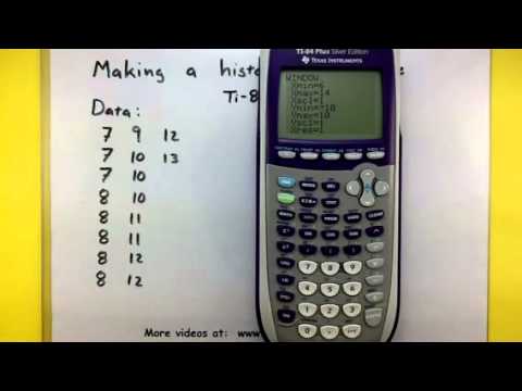
Histograms with a Graphing Calculator

The TI83 and TI84 graphing calculators give us a nice and easy way to get a histogram in order to see the overall pattern of a data set (which is the goal of any histogram!). In this guide, we will go the whole process step by step. As we work through this, you might find it useful to download this Histograms on the Calculator Cheat Sheet (PDF) (just right click and select save as).

Example (video example)

12

14

14

14

16 18

20

20

21

23 27

27

27

29

31 31

32

32

34

36 40

40

40

40

40 42

51

56

60

65

Enter your data into a single list. To get to the lists in your calculator, press STAT and then choose 1:EDIT. There are several lists to choose from but L1 is the default list on the other menus. This means that if you use L1, you will have less stuff to change in the calculator later. To enter data, type the number and then press ENTER. Again, it is really important that all of the data goes into one list – even if in your book it is in different columns.

Go into StatPlots and Select the Histogram Once the data is entered, press 2ND and then Y= to get in the statplot menu. Under this menu, go into plot 1 (you can use any plot, but again, this is the easiest to work with) and turn the plot on. Once the plot is on, select the histogram by highlighting it and pressing enter, and make sure the list says L1. If you used a different list, you will have to change the list here. Finally, leave “frequency” as 1.

Use ZOOMSTAT to view your histogram and TRACE to see the classes and frequency. Once your plot is on, press ZOOM and then #9 ZOOMSTAT to see your graph. The TRACE button allows you to see what the groups/classes are and the frequency. Often, the class width the calculator uses isn’t very natural. In this example its 8.8. It’s a good idea to change this to something that is easier to work with and in this example I decided to change this to 9. To do this, you press WINDOW and adjust the number next to XSCL. Once you do this, press GRAPH to see your changes since pressing ZOOMSTAT will make the calculator recalculate everything.

In the last image, “n” is the frequency of the class denoted by the two numbers in the inequality. For example, the highlighted class in the last picture goes from 12 to 21 and has a frequency of 8.

The video below will walk you through the same example above. Review this to make sure you understand how this all works!

What if there is an error?

If you get all the way to the end and then your graph won’t show up, I would make sure there is nothing under “Y=”. Sometimes when you walk around, your calculator accidentally gets turned on and a bunch of stuff can get pressed and typed under Y=. If this doesn’t fix it, I would then make sure everything is under L1 and not some other list. You can reset your list by clicking STAT, EDIT, SETUPEDITOR if you have a weird menu.

Other Articles

If you are just learning about histograms, you may want to read about how to find them completely by hand.

Want More In Depth Info? Download the “Statistical Plots on the TI83/84” for a step-by-step guide to every type of plot you might want to make on the calculator. DOWNLOAD GUIDE

Subscribe to our Newsletter! We are always posting new free lessons and adding more study guides, calculator guides, and problem packs. Sign up to get occasional emails (once every couple or three weeks) letting you know what’s new! SUBSCRIBE

So you have finished reading the how to get histogram on ti 84 plus topic article, if you find this article useful, please share it. Thank you very much. See more: how to graph histogram on calculator, how to change bin width on ti-84, how to make a boxplot on ti-84, how to make a relative frequency histogram on a ti-84, how to make a histogram, ti-84 histogram invalid dim, histogram graphing calculator, frequency distribution ti-84

Top 27 How To Get Histogram On Ti 84 Plus 455 People Liked This Answer

How do you graph a relative frequency histogram on a TI 84?

How do you plot a histogram?

How do you graph stats on a TI 84?

How do you reset a TI 84 Plus calculator?

What is a frequency histogram?

Is histogram and bar graph the same?

How do you draw a histogram for grouped data?

How do you make a Boxplot on TI 84?

What is a frequency histogram?

TI-84: Histograms | TI-84 Graphing Calculator | CPM Student Tutorials

Making Histograms with a TI-84 Plus & Manually Adjusting Classes – YouTube

Statistics – How to make a histogram using the TI-83/84 calculator – YouTube

TI-84: Histograms | TI-84 Graphing Calculator | CPM Student Tutorials

Graphing Data: Histograms | SparkNotes

How to Construct Histograms on the TI-84 Plus Article – dummies

Histograms with a Graphing Calculator

how to get histogram on ti 84 plus

how to get histogram on ti 84 plus

Probability Histograms

Graphing Data: Histograms

How to Construct Histograms on the TI-84 Plus Article

Adjusting the class size of a histogram

Adjusting the class size of a histogram

Histograms with a Graphing Calculator

Leave a Comment Cancel reply