
Contents
Make a Histogram Using Excel’s Histogram tool in the Data Analysis ToolPak
นอกจากการดูบทความนี้แล้ว คุณยังสามารถดูข้อมูลที่เป็นประโยชน์อื่นๆ อีกมากมายที่เราให้ไว้ที่นี่: ดูความรู้เพิ่มเติมที่นี่
We will create a Histogram in Excel using the Histogram tool in the Data Analysis ToolPak, and we will let Excel choose the number of classes/bins to use.
Excel Histogram with Normal Distribution Curve
Excel Histogram with Normal Distribution Curve
In this video, we will explain how you can create a histogram with a normal distribution curve in Excel.
0:00 Excel Histogram with Normal Distribution Curve Intro
0:44 Creating Histogram Table using Analysis Toolpak
2:31 Inserting the Histogram
4:22 Inserting the Normal Distribution Curve
https://softtechtutorials.com/microsoftoffice/excel/excelhistogramwithnormaldistributioncurve/
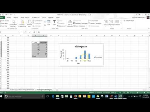
Before we can ask Excel to insert the table, we first need to define the bins. Here we choose to start at 150 and then jump by 5 up to 200. Now we navigate to Data and select Data Analysis. A menu opens where we select Histogram, we press on OK and the Histogram menu opens.
Now we are ready to start creating the histogram and normal distribution curve. First, we select the histogram data, navigate to Insert, and select Scatter with Smooth Lines and Markers. The graph appears on the screen.
Next, we adjust the xaxis such that the curve is bigger and more centered on the screen. We doubleclick on the xaxis such that the Format Axis panel opens. Here, you go to the three bars icon, click on Axis Options and change the minimum and maximum to whatever suits you.
In the next step, we click on Add Chart Element, Error Bars, and More Error Bars Options. The Format Error Bars panel opens and you click on the three bars icon. Here, you select Minus, No Cap, Percentage, and set Percentage to 100.
We only need to remove the curve from the chart before we start with creating the normal distribution curve. To remove the curve, we click on it. This opens the Format Data Series panel. Here, we can select No line in the Line section. Under Marker, we navigate to Marker Options and select None.
Let’s start adding the normal distribution curve. To construct the curve, we first must define the data points. We will compute the corresponding yvalues to the xvalues between 145 and 205 as this covers the entire xrange of the histogram.
To compute the corresponding yvalues, we first use the NORM.DIST function to compute the normal probability distribution curve. So, we type equals NORM.DIST of the xvalue, mean, standard deviation and finally we insert FALSE to indicate we want the probability and not the cumulative distribution function.
Now we are ready to add the normal distribution curve to the chart. This can be done by selecting the graph, then Chart Design, and pressing on Select Data. We click on Add, insert the xvalues and yvalues and press on OK.
To change this, we insert a new column and add the midpoints of the bins instead of the endpoints. Next, we click on the histogram and drag the purple square representing the xvalues to the midpoints. The graph is now how we want.
This concludes our tutorial on Excel Histogram with normal distribution curve. I’m inspired by content creators as Leila Gharani and Teacher’s Tech.
Excel Tutorials Statistics

🌟 EXCEL 7 QC 🌟 5. Biểu đồ phân bố Histogram
File Excel download https://www.fshare.vn/file/1A134ZEQAU6Y
5h17PM Học trò Phạm Ngọc Thành

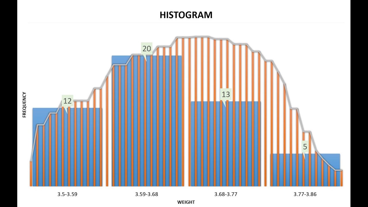
Excel thống kê cơ bản Bài 4 Histogram phân bố trọng lượng
https://www.fshare.vn/file/Z2YH53PZNWEX
11h15 ngày 13102016 … Ngày này năm ấy. Đêm 12102015 trong hào khí nức lòng người. Cả nhà quây quần ngồi bệt trên những manh chiếu cói. Vẽ rạng rỡ sáng ngời trên những khuôn mặt có đôi phần hốc hác sau những ngày khẩn trương chuẩn bị … nhiều cái giọng nói khàn đục, cất không nên lời sau những ngày xuyên đêm. Những lúc mệt nhoài, ngã lưng xuống, tất cả chúng ta đã chợp mắt bên nhau … Tỉnh dậy 1 tí là hào khí xông lên lao vào chiến cuộc …
Tất cả cho 1 ngày 13102015 … Đúng 5h sáng ngày 13102015 … Cả nhà sáng đèn … ánh sáng tỏa ra trong từng ánh mắt … tiếng bước chân nhộn nhịp rộn rã … từ trên lầu đến dưới đất … Những ánh mắt biết cười lan tõa như những làn sóng nhẹ nhàng giao thoa vào nhau …
Gần như điều huyền diệu … một phép màu … những chiếc găng nóng hổi đầu tiên được chuyền tay nhau trong niềm hạnh phúc rạng ngời … Mẽ găng đầu tiên … Chúng ta đã sản xuất được…
Vâng ngay từ Mẽ găng đầu tiên … những chiếc găng được nâng niu trong tay … mềm mại, dẽo dai … đầy sức quyến rũ thôi miên tất cả những ánh mắt … những con tim Gang Viet Family.
10 tiếng … 48h … Cả nhà đã viết nên huyền thoại về một cuộc chinh phục …
Gang Viet Gang Viet
… Lung linh lung linh 2 tiếng gia đình …
Lịch sum họp đoàn tựu gia đình, nghỉ Tết 15 ngày cả 2 Gia đình Gang Viet va Gia đinh Khai Hoan bắt đầu nghỉ từ 25 Tết ngày 22/1/2017 đến hết Mùng 9 ngày 5/2/2017.
Khai trương Mùng 10 Tết ngày 6/2/1017 lúc 5h sáng.
Phạm Ngọc Thành
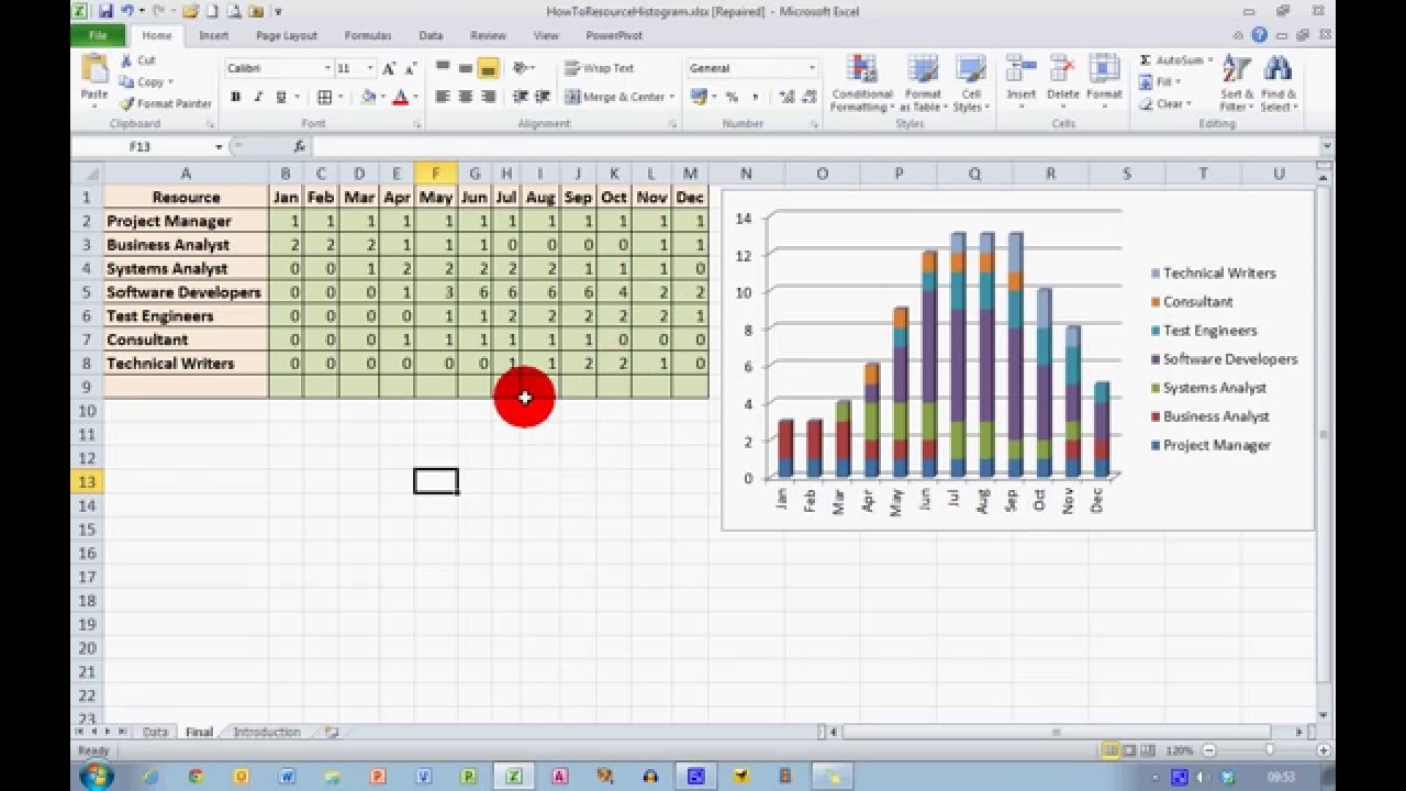
How To… Create a Resource Histogram in Excel 2010
Learn how to create a simple resource histogram in Excel 2010. In this video we use an example of resources required for a Software development project.
นอกจากการดูหัวข้อนี้แล้ว คุณยังสามารถเข้าถึงบทวิจารณ์ดีๆ อื่นๆ อีกมากมายได้ที่นี่: ดูวิธีอื่นๆWIKI