
당신은 주제를 찾고 있습니까 “macrofinancial history and the new business cycle facts – Macrofinancial History and the New Business Cycle Facts“? 다음 카테고리의 웹사이트 https://chewathai27.com/you 에서 귀하의 모든 질문에 답변해 드립니다: https://chewathai27.com/you/blog. 바로 아래에서 답을 찾을 수 있습니다. 작성자 NBER 이(가) 작성한 기사에는 조회수 59회 및 871412 Like 개의 좋아요가 있습니다.
macrofinancial history and the new business cycle facts 주제에 대한 동영상 보기
여기에서 이 주제에 대한 비디오를 시청하십시오. 주의 깊게 살펴보고 읽고 있는 내용에 대한 피드백을 제공하세요!
d여기에서 Macrofinancial History and the New Business Cycle Facts – macrofinancial history and the new business cycle facts 주제에 대한 세부정보를 참조하세요
Macrofinancial History and the New Business Cycle Facts
31st Annual Conference on Macroeconomics
https://www.nber.org/conferences/31st-annual-conference-macroeconomics-2016
Òscar Jordà, Federal Reserve Bank of San Francisco
April 15, 2016
macrofinancial history and the new business cycle facts 주제에 대한 자세한 내용은 여기를 참조하세요.
Macrofinancial History and the New Business Cycle Facts
Macrofinancial History and the New Business Cycle Facts. Oscar Jorda. Federal Reserve Bank of San Francisco. University of California, Davis.
Source: www.frbsf.org
Date Published: 3/1/2022
View: 2859
Macrofinancial History and the New Business Cycle Facts
What are the features of the modern business cycle? Output expansions have almost tripled after World War II, from 3.1 to 8.6 years, whereas credit expansions …
Source: www.journals.uchicago.edu
Date Published: 1/29/2022
View: 3994
Macrofinancial History and the New Business Cycle Facts
More financialized economies exhibit somewhat less real volatility, but also lower growth, more tail risk, as well as tighter real-real and real …
Source: www.nber.org
Date Published: 11/7/2021
View: 2347
Macrofinancial History and the New Business … – IDEAS/RePEc
Òscar Jordà & Moritz Schularick & Alan M. Taylor, 2017. “Macrofinancial History and the New Business Cycle Facts,” NBER Macroeconomics Annual, University of …
Source: ideas.repec.org
Date Published: 12/2/2022
View: 9258
Macrofinancial History and the New Business Cycle Facts
Specifically, they find that joint fluctuations in raw credit, credit-to-GDP and property prices are a strong predictor of financial crises.
Source: www.researchgate.net
Date Published: 1/22/2021
View: 9219
Macrofinancial history and the new business cycle facts – EconBiz
Macrofinancial history and the new business cycle facts. Oscar Jorda (Federal Reserve Bank of San Francisco, University of California, Davis), …
Source: www.econbiz.de
Date Published: 10/24/2022
View: 3385
Macrofinancial History and the New Business Cycle Facts
In advanced economies, a century-long near-stable ratio of credit to GDP gave way to rap financialization and surging leverage in the last …
Source: papers.ssrn.com
Date Published: 7/10/2021
View: 4976
Macrofinancial History and the New Business Cycle Facts
Access a free summary of Macrofinancial History and the New Business Cycle Facts, by Oscar Jorda et al. and 25000 other business, leadership and nonfiction …
Source: www.getabstract.com
Date Published: 10/24/2022
View: 3942
MACROFINANCIAL HISTORY AND THE NEW BUSINESS …
Jordà, Òscar, Moritz Schularick, and Alan M. Taylor. 2018. “MACROFINANCIAL HISTORY AND THE NEW BUSINESS CYCLE FACTS.
Source: conferences.wcfia.harvard.edu
Date Published: 7/23/2021
View: 2764
주제와 관련된 이미지 macrofinancial history and the new business cycle facts
주제와 관련된 더 많은 사진을 참조하십시오 Macrofinancial History and the New Business Cycle Facts. 댓글에서 더 많은 관련 이미지를 보거나 필요한 경우 더 많은 관련 기사를 볼 수 있습니다.
주제에 대한 기사 평가 macrofinancial history and the new business cycle facts
- Author: NBER
- Views: 조회수 59회
- Likes: 871412 Like
- Date Published: 2022. 7. 15.
- Video Url link: https://www.youtube.com/watch?v=PO4k71eaeNY
What are the key business cycle facts?
A cycle consists of expansions occurring at about the same time in many economic activ- ities, followed by similarly general recessions, contractions and revivals which merge into the expansion phase of the next cycle; this sequence of changes is recur- rent but not periodic; in duration business cycles vary from more …
What is the historical cause of the business cycle?
The business cycle is caused by the forces of supply and demand—the movement of the gross domestic product GDP—the availability of capital, and expectations about the future. This cycle is generally separated into four distinct segments: expansion, peak, contraction, and trough.
What is the 4 business cycles and explain each?
business cycle, the series of changes in economic activity, has four stages—expansion, peak, contraction, and trough. Expansion is a period of economic growth: GDP increases, unemployment declines, and prices rise. The peak marks the end of an expansion and the beginning of the next stage, the contraction.
Who created the business cycle?
Business cycles as we know them today were first identified and analyzed by Arthur Burns and Wesley Mitchell in their 1946 book, Measuring Business Cycles. One of their key insights was that many economic indicators move together.
What are the five causes of business cycles?
- 1] Changes in Demand. Keynes economists believe that a change in demand causes a change in the economic activities. …
- Browse more Topics under Business Cycles. …
- 2] Fluctuations in Investments. …
- 3] Macroeconomic Policies. …
- 4] Supply of Money. …
- 1] Wars. …
- 2] Technology Shocks. …
- 3] Natural Factors.
What are the effects of business cycle?
Impact of business cycle on economy
A volatile business cycle is considered bad for the economy. A period of economic boom (rapid growth in GDP) invariably leads to inflation with various economic costs. This inflationary growth tends to be unsustainable and leads to a bust (recession).
Why is the business cycle important?
Understanding business cycles allows owners to make informed business decisions. By keeping a finger on the economy’s pulse and paying attention to current economic projections, they can speculate when to prepare for a contraction and take advantage of the expansion.
What business cycle are we currently in?
Key takeaways
The US and other major economies remain in the mid-cycle phase of the business cycle, but an increasing number of indicators suggest that the late cycle when economic growth slows may be approaching.
How long does a business cycle last?
The length of business cycles varies depending on the economy’s status. The average length of an expansion is a little under five years, and the average length of a contraction is 11 months. The average overall cycle length is 5-1/2 years.
What is the meaning of business cycle?
Business cycles are a type of fluctuation found in the aggregate economic activity of a nation — a cycle that consists of expansions occurring at about the same time in many economic activities, followed by similarly general contractions (recessions). This sequence of changes is recurrent but not periodic.
What is business cycle easy words?
A business cycle is the natural expansion and contraction of economic growth that happens in an economy over a period of time. The rise and fall of an economy’s gross domestic product (GDP) defines the start and end of a business cycle, which is also known as an economic cycle or a trade cycle.
What are the theories of business cycle?
Keynes has proposed three types of propensities to understand business cycles. These are propensity to save, propensity to consume, and propensity of marginal efficiency of capital. He has also developed a concept of multiplier that represents changes in income level produced by the changes in investment.
How many business cycles are there?
Key Takeaways
The business cycle goes through four major phases: expansion, peak, contraction, and trough.
What is the purpose of the business cycle?
The purpose of a business cycle is to track economic activity. In practical terms, the business cycle tracks the state of an economy from expansion to contraction and recession. It can affect how you spend, how you invest, and how you access credit.
What is a business cycle and why is it important?
The business cycle is a pattern of economic booms and busts exhibited by the modern economy. Business cycles are important because they can affect profitability, which ultimately determines whether a business succeeds.
What are the types of business cycle?
There are two types of business cycle: The classical cycle refers to rises and falls in total production. The growth cycle is concerned with fluctuations in the growth rate of production.
What are the phases of business cycle?
Throughout its life, a business cycle goes through four identifiable phases: expansion, peak, contraction, and trough.
Macrofinancial History and the New Business Cycle Facts: NBER Macroeconomics Annual: Vol 31
In advanced economies, a century-long, near-stable ratio of credit to GDP gave way to rapid financialization and surging leverage in the last forty years. This “financial hockey stick” coincides with shifts in foundational macroeconomic relationships beyond the widely noted return of macroeconomic fragility and crisis risk. Leverage is correlated with central business cycle moments, which we can document thanks to a decade-long international and historical data collection effort. More financialized economies exhibit somewhat less real volatility, but also lower growth, more tail risk, as well as tighter real-real and real-financial correlations. International real and financial cycles also cohere more strongly. The new stylized facts that we discover should prove fertile ground for the development of a new generation of macroeconomic models with a prominent role for financial factors.
“When you combine ignorance and leverage, you get some pretty interesting results.” —Warren Buffett
I. Introduction Observation is the first step of the scientific method. This paper lays empirical groundwork for macroeconomic models that take finance seriously. The global financial crisis reminded us that financial factors play an important role in shaping the business cycle, and there is growing agreement that new and more realistic models of real financial interactions are needed. Crafting such models has become one of the top challenges for macroeconomic research. Policymakers in particular seek a better understanding of the interaction between monetary, macroprudential, and fiscal policies. Our previous research (Schularick and Taylor 2012; Jordà, Schularick, and Taylor 2011, 2013, 2016a, 2016b) uncovered a key stylized fact of modern macroeconomic history that we may call the “financial hockey stick.” The ratio of aggregate private credit to income in advanced economies has surged to unprecedented levels over the second half of the twentieth century. A central aim of this paper is to show that, alongside this great leveraging, key business cycle moments have become increasingly correlated with financial variables. Most importantly, our long-run data provide evidence that high-credit economies may not be especially volatile, but their business cycles tend to be more negatively skewed. In other words, leverage is associated with dampened business cycle volatility, but more spectacular crashes. Business cycle outcomes become more asymmetric in high-credit economies, echoing previous research on the asymmetry of cycles (McKay and Reis 2008). A great deal of modern macroeconomic thought has relied on the small (and unrepresentative) sample of US post–World War II experience to formulate, calibrate, and test models of the business cycle; to calculate the welfare costs of fluctuations; and to analyze the benefits of stabilization policies. Yet the historical macroeconomic cross-country experience is richer. An important contribution of this paper is to introduce a new comprehensive macrofinancial historical database covering 17 advanced economies over the last 150 years.1 This considerable data-collection effort has occupied the better part of a decade and involved a small army of research assistants. We see two distinct advantages of using our data. First, models ostensibly based on universal economic mechanisms of the business cycle must account for patterns seen across space and time. Second, a very long-run perspective is necessary to capture enough “rare events” such as major financial dislocations and “macroeconomic disasters” to robustly analyze their impact on the volatility and persistence of real economic cycles. We begin by deconstructing the financial hockey stick. The central development of the second half of the twentieth century is the rise of household credit, mostly of mortgages. Business credit has increased as well, but at a slower pace. Home-ownership rates have climbed in almost every industrialized economy and, with them, real house prices. Private credit has increased much faster than income. Even though households are wealthier, private credit has grown faster even than the underlying wealth. Households are more levered than at any time in history. Next, we characterize the broad contours of the business cycle. Using a definition of turning points similar to many business cycle dating committees, such as the NBER’s, we investigate features of the business cycle against the backdrop of the financial cycle. The associations we present between credit and the length of the expansion, and between deleveraging and the speed of the recovery, already hint at the deeper issues requiring further analysis. Economies grow more slowly and generally more stably post–World War II. Despite this apparent stability, financial crises since the fall of Bretton Woods still occur with devastating regularity. These broad contours lead us to a reevaluation of conventional stylized facts on business cycles using our newer and more comprehensive data, with a particular emphasis on real financial interactions. The use of key statistical moments to describe business cycles goes back at least to the New Classical tradition that emerged in the 1970s (e.g., Kydland and Prescott 1990; Zarnowitz 1992; Backus and Kehoe 1992; Hodrick and Prescott 1997; Basu and Taylor 1999). Under this approach, the statistical properties of models are calibrated to match empirical moments in the data such as means, variances, correlations, and autocorrelations. In the final part of the paper, we examine key business cycle moments conditional on aggregate private-credit levels. We find that rates of growth, volatility, skewness, and tail events all seem to depend on the ratio of private credit to income. Moreover, key correlations and international cross correlations appear to also depend quite importantly on this leverage measure. Business cycle properties have changed with the financialization of economies, especially in the postwar upswing of the financial hockey stick. The manner in which macroeconomic aggregates correlate with each other has evolved as leverage has risen. Credit plays a critical role in understanding aggregate economic dynamics.
II. A New Data Set for Macrofinancial Research The data featured in this paper represent one of its main contributions. We have compiled, expanded, improved, and updated a long-run macrofinancial data set that covers 17 advanced economies since 1870 on an annual basis. The first version of the data set, unveiled in Jordà et al. (2011) and Schularick and Taylor (2012), covered core macroeconomic and financial variables for 14 countries. The latest vintage covers 17 countries and 25 real and nominal variables. Among these, there are time series that had been hitherto unavailable to researchers, especially for key financial variables such as bank credit to the nonfinancial private sector (aggregate and disaggregate) and asset prices (equities and housing). We have now brought together in one place macroeconomic data that previously had been dispersed across a variety of sources. This data set is publicly available at the NBER website. Table 1 gives a detailed overview of the coverage of the latest vintage of the data set, which gets updated on a regular basis as more data are unearthed and as time passes. More details about the data construction appear in an extensive 100-page online appendix, which also acknowledges the support we received from colleagues all over the world. Table 1. A New Macrofinancial Data Set (Available Samples Per Variable and Per Country) Country RGDPpc PPPGDPpc NGDP Population RCons. Inv. Curr. Acc. Exports Imports Gov. Exp. Gov. Rev. CPI Nrw. Mon. Australia 1870–2013 1870–2013 1870–2013 1870–2013 1901–2013 1870–1946 1870–2013 1870–1913 1870–1913 1902–2013 1902–2013 1870–2013 1870–2013 1949–2013 1915–2013 1915–2013 Belgium 1870–2013 1870–2013 1870–1913 1870–2013 1913–2013 1900–1913 1870–1913 1870–1913 1870–1913 1870–1912 1870–1912 1870–1914 1877–1913 1920–1939 1920–1939 1919–2013 1919–2013 1919–2013 1920–1939 1920–2013 1920–1939 1920–1940 1946–2013 1941 1941–2013 1945–2013 1947–2013 1943 1946–2013 Canada 1870–2013 1870–2013 1870–2013 1870–2013 1871–2013 1871–2013 1870–1945 1870–2013 1870–2013 1870–2013 1870–2013 1870–2013 1871–2013 1948–2013 Switzerland 1870–2013 1870–2013 1870–2013 1870–2013 1870–2013 1870–1913 1921–1939 1885–2013 1885–2013 1871–2013 1870–2013 1870–2013 1870–2013 1948–2013 1948–2013 Germany 1870–2013 1870–2013 1870–1944 1870–2013 1870–2013 1870–1913 1872–1913 1872–1913 1872–1913 1872–1913 1873–1915 1870–2013 1876–1913 1946–2013 1920–1939 1925–1938 1924–1943 1924–1943 1925–1938 1925–1938 1924–1938 1948–2013 1948–2013 1948–2013 1948–2013 1950–2013 1950–2013 1951–2011 Denmark 1870–2013 1870–2013 1870–2013 1870–2013 1870–2013 1870–1914 1874–1914 1870–2013 1870–2013 1870–1935 1870–1935 1870–2013 1870–1945 1922–2013 1921–2013 1937–2013 1954–2013 1950–2013 Spain 1870–2013 1870–2013 1870–2013 1870–2013 1870–2013 1870–2013 1870–1913 1870–1935 1870–1935 1870–1935 1870–1935 1880–2013 1874–1935 1931–1934 1939–2013 1939–2013 1940–2013 1940–2013 1941–2011 1940–2013 Finland 1870–2013 1870–2013 1870–2013 1870–2013 1870–2013 1870–2013 1870–2013 1870–2013 1870–2013 1882–2013 1882–2013 1870–2013 1870–2013 France 1870–2013 1870–2013 1870–1913 1870–2013 1870–2013 1870–1918 1870–1913 1870–2013 1870–2013 1870–2013 1870–2013 1870–2013 1870–1913 1920–1938 1920–1944 1919–1939 1920–2013 1950–2013 1946–2013 1948–2013 UK 1870–2013 1870–2013 1870–2013 1870–2013 1870–2013 1870–2013 1870–2013 1870–2013 1870–2013 1870–2013 1870–2013 1870–2013 1870–2013 Italy 1870–2013 1870–2013 1870–2013 1870–2013 1870–2013 1870–2013 1870–2013 1870–2013 1870–2013 1870–2013 1870–2013 1870–2013 1870–2013 Japan 1870–2013 1870–2013 1875–1944 1870–2013 1874–2013 1885–1944 1870–1944 1870–1943 1870–1943 1870–2013 1870–2013 1870–2013 1873–2013 1946–2013 1946–2013 1946–2013 1946–2013 1946–2013 Netherlands 1870–2013 1870–2013 1870–1913 1870–2013 1870–2013 1870–1913 1870–1913 1870–1943 1870–1943 1870–2013 1870–2013 1870–2013 1870–1941 1921–1939 1921–1939 1921–1939 1946–2013 1946–2013 1945–2013 1945–2013 1948–2013 1948–2013 Norway 1870–2013 1870–2013 1870–1939 1870–2013 1870–2013 1870–1939 1870–1939 1870–2013 1870–2013 1870–2013 1870–1943 1870–2013 1870–2013 1946–2013 1946–2013 1946–2013 1949–2013 Portugal 1870–2013 1870–2013 1870–2013 1870–2013 1910–2013 1953–2013 1870–2013 1870–2013 1870–2013 1870–2013 1870–2013 1870–2013 1870–2013 Sweden 1870–2013 1870–2013 1870–2013 1870–2013 1870–2013 1870–2013 1870–2013 1870–2013 1870–2013 1870–2013 1870–2013 1870–2013 1871–2013 USA 1870–2013 1870–2013 1870–2013 1870–2013 1870–2013 1870–2013 1870–2013 1870–2013 1870–2013 1870–2013 1870–2013 1870–2013 1870–2013 Country Broad Mon. S.t. Rate L.t. Rate Stocks Ex. Rate Pub. Debt Bank Lend. Mort. Lend. Hh. Lend. Bus. Lend. H. Prices Bk. Crisis Australia 1870–2013 1870–1944 1870–2013 1870–2013 1870–2013 1870–2013 1870–1945 1870–1945 1870–1945 1870–1945 1870–2013 1870–2013 1948–2013 1948–2013 1952–2013 1952–2013 1952–2013 Belgium 1979–2013 1870–1914 1870–1912 1870–2013 1870–2013 1870–1913 1885–1913 1885–1913 1950–2013 1950–2013 1878–1913 1870–2013 1920–2013 1920–2013 1920–1939 1920–1940 1920–1939 1919–2013 1946–1979 1950–2013 1950–2013 1982–2013 Canada 1871–2013 1934–1944 1870–2013 1870–2013 1870–2013 1870–2013 1870–2013 1874–2013 1956–2013 1961–2013 1921–1949 1870–2013 1948–2013 1956–2013 Switzerland 1880–2013 1870–2013 1880–2013 1899–1914 1870–2013 1880–2013 1870–2013 1870–2013 1870–2013 1870–2013 1901–2013 1870–2013 1916–2013 Germany 1880–1913 1870–1914 1870–1921 1870–1921 1870–1944 1871–1913 1883–1920 1883–1919 1950–2013 1950–2013 1870–1922 1870–2013 1925–1938 1919–1922 1924–1943 1924–2013 1946–2013 1927–1943 1924–1940 1924–1940 1924–1938 1924–1944 1948–2013 1950–2013 1946–2013 1949–2013 1962–2013 1949–2013 1950–2013 Denmark 1870–1945 1875–2013 1870–2013 1892–2013 1870–2013 1880–1946 1870–2013 1875–2013 1951–2013 1951–2013 1875–2013 1870–2013 1950–2013 1953–1956 1960–1996 1998–2013 Spain 1874–1935 1883–1914 1870–1936 1870–2013 1870–2013 1880–1935 1900–1935 1904–1935 1946–2013 1946–2013 1971–2013 1870–2013 1941–2013 1920–2013 1940–2013 1940–2013 1946–2013 1946–2013 Finland 1870–2013 1870–2013 1870–1938 1912–2013 1870–2013 1914–2013 1870–2013 1927–2013 1948–2013 1948–2013 1905–2013 1870–2013 1948–2013 France 1870–1913 1870–1914 1870–2013 1870–2013 1870–2013 1880–1913 1900–1938 1870–1933 1958–2013 1958–2013 1870–2013 1870–2013 1920–2013 1922–2013 1920–1938 1946–2013 1946–2013 1949–2013 UK 1870–2013 1870–2013 1870–2013 1870–2013 1870–2013 1870–2013 1880–2013 1880–2013 1880–2013 1880–2013 1899–1938 1870–2013 1946–2012 Italy 1880–2013 1885–1914 1870–2013 1906–2013 1870–2013 1870–2013 1870–2013 1870–2013 1950–2013 1950–2013 1870–2013 1870–2013 1922–2013 Japan 1894–2013 1879–1938 1870–2013 1878–1891 1870 1875–1944 1874–2013 1893–1940 1948–2013 1948–2013 1913–1930 1870–2013 1957–2013 1893–2013 1873–2013 1946–2013 1946–2013 1936–2013 Netherlands 1870–1941 1870–1914 1870–2013 1890–1944 1870–2013 1870–1939 1900–2013 1900–2013 1990–2013 1990–2013 1870–2013 1870–2013 1945–2013 1919–1944 1946–2013 1946–2013 1948–2013 Norway 1870–2013 1870–1965 1870–2013 1914–2013 1870–2013 1880–1939 1870–2013 1870–2013 1978–2013 1978–2013 1870–2013 1870–2013 1967–2013 1947–2013 Portugal 1913–2013 1880–2013 1870–2013 1929–2013 1870–2013 1870–2013 1870–1903 1920–2013 1979–2013 1979–2013 1988–2013 1870–2013 1920–2013 Sweden 1871–2013 1870–2013 1870–2013 1870–2013 1870–2013 1870–2013 1871–2013 1871–2013 1871–1940 1975–2013 1875–2013 1870–2013 1975–2013 USA 1870–2013 1870–2013 1870–2013 1871–2013 1870–2013 1870–2013 1880–2013 1880–2013 1945–2013 1945–2013 1890–2013 1870–2013 In addition to country experts, we consulted a broad range of sources such as economic and financial history volumes and journal articles, and various publications of statistical offices and central banks. For some countries we extended existing data series from previous statistical work of financial historians or statistical offices. This was the case for Australia, Canada, Japan, and the United States. For other countries we chiefly relied on recent data collection efforts at central banks such as for Denmark, Italy, and Norway. Yet in a non-negligible number of cases we had to go back to archival sources including documents from governments, central banks, and private banks. Typically, we combined information from various sources and spliced series to create long-run data sets spanning the entire 1870–2014 period for the first time.
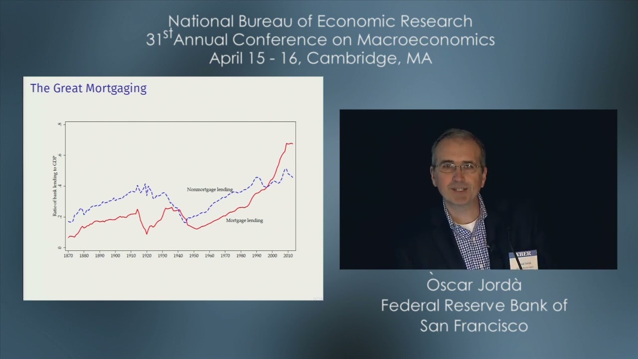
III. The Financial Hockey Stick The pivotal feature to emerge in the last 150 years of global macroeconomic history, as was first highlighted in Schularick and Taylor (2012), is the “hockey stick” pattern of private credit in advanced economies displayed in figure 1. Focusing on private credit, defined henceforth as bank lending to the nonfinancial private sector, we can see that this variable maintained a relatively stable relationship with gross domestic product (GDP) and broad money until the 1970s. After an initial period of financial deepening in the nineteenth century, the average level of the credit-to-GDP ratio in advanced economies reached about 50%–60% around 1900. With the exception of the deep contraction in bank lending that was seen from the crisis of the Great Depression to World War II, the ratio was stable in this range until the 1970s. Fig. 1. The financial hockey stick Note: Total loans is bank lending to the nonfinancial private sector, broad money is M2 or similar broad measure of money, both expressed as a ratio to GDP averaged over the 17 countries in the sample (see text). Throughout this chapter we use the term “leverage” to denote the ratio of private credit to GDP. Although leverage is often used to designate the ratio of credit to the value of the underlying asset or net worth, income leverage is equally important, as debt is serviced out of income. Net-worth-leverage is more unstable due to fluctuations in asset prices. For example, at the peak of the recent US housing boom, ratios of debt to housing wealth signaled that household leverage was declining just as ratios of debt to income were exploding (Foote, Gerardi, and Willen 2012). Similarly, corporate balance sheets based on market values may mislead: in 2006–07 overheated asset values indicated robust capital ratios in major banks that were in distress or outright failure a few months later. In the past four decades, the volume of private credit has grown dramatically relative to both output and monetary aggregates, as shown in figure 1. The disconnect between private credit and (traditionally measured) monetary aggregates has resulted, in large part, from the shrinkage of bank reserves and the increasing reliance by financial institutions on nonmonetary means of financing, such as bond issuance and interbank lending. Private credit in advanced economies doubled relative to GDP between 1980 and 2009, increasing from 62% in 1980 to 118% in 2010. The data also demonstrate the breathtaking surge of bank credit prior to the global financial crisis in 2008. In a little more than 10 years, between the mid-1990s and 2008–09, the average bank credit-to-GDP ratio in advanced economies rose from a little under 80% of GDP in 1995 to more than 110% of GDP in 2007. This 30 percentage points (pps) increase is likely to be a lower bound estimate as credit creation by the shadow banking system, of considerable size in the United States and to a lesser degree in the United Kingdom, is excluded from our banking-sector data. What has been driving this great leveraging? A look at the disaggregated credit data, discussed in greater detail in Jordà, Schularick, and Taylor (2015), shows that the business of banking evolved substantially over the past 140 years. Figure 2 tracks the development of bank lending to the nonfinancial corporate sector and lending to households for our sample of 17 advanced economies. The ratio of business lending relative to GDP has remained relatively stable over the past century. On the eve of the global financial crisis, bank credit to corporates was not meaningfully higher than on the eve of World War I. Fig. 2. Bank lending to business and households Note: Business loans and household loans are expressed as a ratio to GDP averaged over the 17 countries in the sample (see text). Figure 3 tracks the evolution of mortgage and nonmortgage lending (mostly unsecured lending to businesses) relative to GDP from 1870 to the present. The graph demonstrates that mortgage borrowing has accelerated markedly in the advanced economies after World War II, a trend that is common to almost all individual economies. Mortgage lending to households accounts for the lion’s share of the rise in credit-to-GDP ratios in advanced economies since 1980. To put numbers on these trends: at the turn of the nineteenth century, mortgage credit accounted for less than 20% of GDP on average. By 2010, mortgage lending represented 70% of GDP, more than three times the historical level at the beginning of the twentieth century. The main business of banks in the early 1900s consisted of making unsecured corporate loans. Today, however, the main business of banks is to extend mortgage credit, often financed with short-term borrowings. Mortgage loans now account for somewhere between one-half and two-thirds of the balance sheet of a typical advanced-country bank. Fig. 3. The great mortgaging Note: Mortgage loans and nonmortgage loans are expressed as a ratio to GDP averaged over the 17 countries in the sample. Mortgage lending is to households and firms. Nonmortgage lending is unsecured lending primarily to businesses (see text). It is true that a substantial share of mortgage lending in the nineteenth century bypassed the banking system and took the form of private lending. Privately held mortgage debt likely accounted for close to 10% of GDP at the beginning of the twentieth century. A high share of farm and nonfarm mortgages was held outside banks in the United States and Germany (Hoffman, Postel-Vinay, and Rosenthal 2000). A key development in the twentieth century was the subsequent transition of these earlier forms of “informal” real estate finance into the hands of banks and the banking system in the course of the twentieth century. Moreover, even as we discuss the key aggregate trends, we do not mean to downplay the considerable cross-country heterogeneity in the data. Table 2 decomposes for each country the increase of total bank lending to GDP ratios over the past 50 years into growth of household debt and business debt as well as secured and unsecured lending. The percentage point change in the ratio of private credit to GDP in Spain was about three times higher than in Japan and more than twice as high as in Germany and Switzerland. However, it is equally clear from the table that the increase in the private credit-to-GDP ratio, as well as the central role played by mortgage credit to households, are both widespread phenomena. Table 2. Change in Bank Lending-to-GDP Ratios (Multiple), 1960–2012 Country Total Lending
(1) Mortgage
(2) Nonmortgage
(3) Households
(4) Business
(5) Netherlands 1.31 0.67 0.63 — — Denmark 1.18 0.98 0.19 0.75 0.43 Australia 1.12 0.72 0.40 0.78 0.34 Spain 1.11 0.78 0.33 0.70 0.41 Portugal 1.01 0.59 0.42 — — USA* 0.82 0.43 0.39 0.40 0.42 USA 0.21 0.17 0.04 0.13 0.07 Sweden 0.76 0.48 0.29 — — Great Britain 0.73 0.51 0.23 0.61 0.12 Canada 0.69 0.39 0.30 0.60 — Finland 0.62 0.27 0.35 0.42 0.19 Switzerland 0.61 0.83 −0.21 0.60 0.01 Italy 0.55 0.49 0.07 0.39 0.16 France 0.54 0.41 0.12 0.41 0.13 Belgium 0.51 0.32 0.19 0.34 0.17 Germany 0.49 0.28 0.21 0.20 0.29 Norway 0.40 0.53 −0.13 — — Japan 0.38 0.41 −0.03 0.28 0.10 Average 0.72 0.52 0.20 0.48 0.20 Fraction of Average 1.00 0.72 0.28 0.71 0.29 The central question that we address in the remainder of the paper is to see if and how this secular growth of finance, the growing leverage of incomes, and the changes in the composition of bank lending have gone hand in hand with changes in the behavior of macroeconomic aggregates over the business cycle.
IV. Household Leverage, Home Ownership, and House Prices A natural question to ask is whether this surge in household borrowing occurred on the intensive or extensive margin. In other words, did more households borrow or did households borrow more? Ideally, we would have long-run household-level data to address this question, but absent such figures we can nonetheless infer some broad trends from our data. If households increased debt levels, not only relative to income but also relative to asset values, this would raise greater concerns about the macroeconomic stability risks stemming from more highly leveraged household portfolios. Historical data for the total value of the residential housing stock (structures and land) are only available for a number of benchmark years. We relate those to the total volume of outstanding mortgage debt to get an idea about long-run trends in real estate leverage ratios. Regarding sources, we combine data from Goldsmith’s (1985) classic study of national balance sheets with recent estimates of wealth-to-income ratios by Piketty and Zucman (2013). Margins of error are wide, as it is generally difficult to separate the value of residential land from overall land for the historical period. We had to make various assumptions on the basis of available data for certain years. Figure 4 shows that the ratio of household mortgage debt to the value of real estate has increased considerably in the United States and the United Kingdom in the past three decades. In the United States, mortgage debt-to-housing value climbed from 28% in 1980 to over 40% in 2013, and in the United Kingdom from slightly more than 10% to 28%. A general upward trend in the second half of the twentieth century is also clearly discernible in a number of other countries. Fig. 4. Ratio of household mortgage lending to the value of the housing stock Figure 5 shows that this upward trend in debt-to-asset ratios coincided with a surge in global house prices, as discussed in Knoll, Schularick, and Steger (2015). Real house prices exhibit a hockey-stick pattern just like the credit aggregates. Having stayed constant for the first century of modern economic growth, global house prices embarked on a steep ascent in the second half of the twentieth century and tripled within three decades of the onset of large-scale financial liberalization. Fig. 5. Real house prices, 1870–2013 Source: Knoll, Schularick, and Steger (2015). Note: Average CPI-deflated house price index for 14 advanced countries. A second trend is equally important: the extensive margin of mortgage borrowing also played a role. Table 3 demonstrates that the rise in economy-wide leverage has financed a substantial expansion of home ownership in many countries. The idea that home ownership is an intrinsic part of the national identity is widely accepted in many countries, but in most cases it is a relatively recent phenomenon. Before World War II, home ownership was not widespread. In the United Kingdom, for instance, home-ownership rates were in the low 20% range in the 1920s. In the United States, the home-ownership rate did not cross the 50% bar until after World War II, when generous provisions in the GI Bill helped push it up by about 10 percentage points. For the sample average, home-ownership rates were around 40% after World War II. By the first decade of the twenty-first century, they had risen to 60%—an increase of about 20 percentage points in the course of the past half century. In some countries, such as Italy, we observe that home-ownership rates doubled after World War II. In others, such as France and the United Kingdom, they went up by nearly 50%. Table 3. Home-Ownership Rates in the Twentieth Century (Owner-Occupied Share of Units, Percent) Canada Germany France Italy Switzerland United Kingdom United States Average 1900 47 1910 46 1920 23 46 1930 48 1940 57 32 44 1950 66 39 38 40 37 32 47 43 1960 66 34 41 45 34 42 62 46 1970 60 36 45 50 29 50 63 48 1980 63 39 47 59 30 58 64 51 1990 63 39 55 67 31 68 64 55 2000 66 45 56 80 35 69 67 60 2013 69 45 58 82 37 64 65 60 Quantitative evidence on the causes of such pronounced differences in home-ownership rates between advanced economies is still scarce. Differences in rental regulation, tax policies, and other forms of government involvement, as well as ease of access to mortgage finance and historical path dependencies, likely all played a role. Studies in historical sociology, such as Kohl (2014), explain differences in home-ownership rates between the United States, Germany, and France, as a consequence of the dominant role played by the organization of urban housing markets. In all countries, the share of owner-occupied housing is roughly comparable in rural areas; rather, the stark differences in aggregate ownership rates are mainly a function of the differences in the organization of urban housing across countries. Divergent trajectories in housing policy also matter. In the United States, the Great Depression was the main catalyst for new policies aimed at facilitating home ownership. Yet government interventions in the housing market remained an important part of the policy landscape after World War II, or even intensified. In the US case, the Veterans Administration (VA) was established through the GI Bill in 1944. The VA guaranteed loans with high loan-to-value ratios over 90%, with some loans passing the 100% loan-to-value mark (Fetter 2013). Forty percent of all mortgages were federally subsidized in the 1950s. The GI Bill is credited with explaining up to one-quarter of the post–World War II increase in the rate of home ownership. In many European countries, the government already took a more active role in the housing sector following World War I. But European housing policies tended to focus on public construction and ownership of housing, whereas in the United States, the emphasis was on financial support for individual home ownership through the subsidization of mortgage interest rates or public loan guarantees. The experience with the Great Depression was also formative with regard to the growing role of the state in regulating and ultimately backstopping the financial sector. The most prominent innovation was deposit insurance. In the United States, deposit insurance was introduced as part of the comprehensive Banking Act of 1933, commonly known as the Glass-Steagall Act. Some European countries like Switzerland and Belgium also introduced deposit insurance schemes in the 1930s. In the majority of European countries deposit insurance was introduced in the decades following World War II, albeit with considerable institutional variety (Demirgüç-Kunt, Kane, and Laeven 2013). However, different American and European approaches to the organization of deposit insurance are observable. This is because, at least in the early stages, European deposit insurance schemes relied chiefly on industry arrangements. The United States stands out as the first country that committed the tax payer to back-stopping the banking system. A common effect of the Depression, however, was that in almost all countries the role of the state as a financial player increased. After the devastating consequences of a dysfunctional financial sector had become apparent during the 1930s, the sector was kept on a short leash. Directly or indirectly, the state became more intertwined with finance. Among the major economies, Germany clearly went to one extreme by turning the financial sector into little more than a handmaiden of larger policy goals in the 1930s. In doing so, it inadvertently pioneered various instruments of financial repression (e.g., channeling deposits into government debt) that, in one form or the other, became part of the European financial policy tool kit after World War II. For instance, France ran a tight system of controls on savings flows in the postwar decades (Monnet 2014). In this long-run context, can we say in any quantitative way the role played by debt-income and debt-wealth changes over time in the evolution of leverage? To this end, figure 6 and Table 4 provide comparisons of borrowing, wealth, and GDP. The figure displays three grand ratios for the average of the United States, United Kingdom, France, and Germany over the post–World War II era in 20-year windows. Panel (a) displays total private lending to the nonfinancial sector (total lending) as a ratio to GDP (solid line), total lending as a ratio to total wealth (dashed line), and total wealth as a ratio to GDP (dotted line). Panel (b) of the same figure presents a similar but more granular decomposition to focus on the housing market: the ratio of mortgages to GDP (solid thick line), the ratio of mortgages to housing wealth (dashed line), and the ratio of housing wealth to GDP (dotted line). Data on wealth come from Piketty and Zucman (2013) and are available only for selected countries and a limited sample. Fig. 6. Leverage—loans, wealth, and income in the United States, United Kingdom, France, and Germany, averages Source: Data on wealth and housing wealth available online at http:piketty.pse.ens.fr/en/capitalisback from Piketty and Zucman (2013). All other data collected by the authors. Note: Variables expressed as ratios. Right-hand-side axes always refer to wealth over GDP ratios. Table 4. Leverage—Grand Ratios for Loans, Wealth, and GDP in the United States, United Kingdom, France, and Germany (Averages and by Country) (a) All Wealth, All Loans (b) Housing Wealth, Mortgage Loans 1950 1970 1990 2010 1950 1970 1990 2010 Loans/GDP US 0.55 0.90 1.2 1.65 0.30 0.44 0.63 0.92 UK 0.23 0.30 0.88 1.07 0.09 0.15 0.38 0.65 France 0.32 0.59 0.79 0.98 0.10 0.19 0.30 0.52 Germany 0.19 0.59 0.87 0.95 0.03 0.25 0.27 0.46 Average 0.32 0.59 0.94 1.16 0.13 0.26 0.40 0.64 Loans/Wealth US 0.14 0.23 0.29 0.38 0.18 0.26 0.35 0.47 UK 0.11 0.09 0.19 0.20 0.08 0.11 0.19 0.21 France 0.11 0.16 0.21 0.16 0.08 0.12 0.16 0.13 Germany 0.08 0.19 0.24 0.23 0.04 0.17 0.14 0.19 Average 0.11 0.17 0.24 0.24 0.09 0.16 0.21 0.25 Wealth/GDP US 3.80 4.00 4.19 4.31 1.70 1.71 1.83 1.94 UK 2.08 3.33 4.62 5.23 1.11 1.44 1.99 3.03 France 2.91 3.63 3.68 6.05 1.30 1.64 1.94 3.83 Germany 2.29 3.13 3.55 4.14 0.91 1.48 1.91 2.39 Average 2.77 3.52 4.01 4.93 1.26 1.57 1.92 2.80 Similarly, table 4 displays these three grand ratios, again organized by the same principles: panel (a), for all categories of lending and wealth; panel (b), for mortgages and housing wealth. The table provides data for the United States, United Kingdom, France, and Germany, as well as the average across all four, which is used to construct figure 6. It should be clear from the definition of these three grand ratios that our concept of leverage, defined as the ratio of lending to GDP, is mechanically linked to the ratio of lending to wealth times the ratio of wealth to GDP. Figure 6 and panel (b) of Table 4, in particular, give a compelling reason to focus on the ratio of mortgages to GDP rather than as a ratio to housing wealth. In the span of the last 60 years, the ratio of mortgages to GDP is nearly six times larger; whereas, measured against housing wealth, mortgages have almost tripled. Of course, the reason for this divergence is the accumulation of housing wealth over the this period, which has more than doubled when measured against GDP. Summing up, our study of the financial hockey stick has yielded three core insights. First, the sharp rise of aggregate credit-to-income ratios is linked mainly to rising mortgage borrowing by households. Bank lending to the business sector has played a subsidiary role in this process and has remained roughly constant relative to income. Second, the rise in aggregate mortgage borrowing relative to income has been driven by substantially higher aggregate loan-to-value ratios against the backdrop of house price gains that have outpaced income growth in the final decades of the twentieth century. Lastly, the extensive margin of increasing home-ownership rates mattered, too. In many countries, home-ownership rates have increased considerably. The financial hockey stick can therefore be understood as a corollary of more highly leveraged home ownership against substantially higher asset prices.
V. Expansions, Recessions, and Credit What are the key features of business and financial cycles in advanced economies over the last 150 years? A natural way to tackle this question is to divide our annual frequency sample into periods of real GDP per capita growth or expansions, and years of real GDP per capita decline or recessions. At annual frequency, this classification is roughly equivalent to the dating of peaks and troughs routinely issued by business cycle committees, such as the NBER’s for the United States. We will use the same approach to discuss cycles based on real credit per capita (measured by our private credit variable deflated with the CPI index). This will allow us to contrast the GDP and credit cycles. This characterization of the cycle does not depend on the method chosen to detrend the data, or on how potential output and its dynamics are determined. Rather, it is based on the observation that in economies where the capital stock and population are growing, negative economic growth represents a sharp deterioration in business activity, well beyond the vagaries of random noise.2 In a recent paper, McKay and Reis (2008) reach back to Mitchell (1927) to discuss two features of the business cycle, “brevity” and “violence,” in Mitchell’s words.3 Harding and Pagan (2002) provide more operational definitions that are roughly equivalent. In their paper, brevity refers to the duration of a cyclical phase, expressed in years. Violence refers to the average rate of change per year. It is calculated as the overall change during a cyclical phase divided by its duration and expressed as percent change per year. These simple statistics, duration (or violence) and rate (or brevity), can be used to summarize the main features of business and credit cycles. Table 5 shows two empirical regularities: (1) the growth cycles in real GDP (per capita) and in real credit growth using turning points in GDP; and (2) the same comparison between GDP and credit, this time using turning points in credit. In both cases, the statistics are reported as an average for the full sample of 17 advanced economies, and for the pre– and post–World War II subsamples. Table 5. Duration and Rate of Change—GDP versus Credit Cycles Expansions Recessions Full Pre-WWII Post-WWII Full Pre-WWII Post-WWII GDP-based cycles Duration (years) 5.1 3.1 8.6 1.5 1.6 1.4 (5.5) (2.7) (7.2) (0.9) (1.0) (0.8) Rate (% p.a) GDP 3.7 4.1 3.0 −2.5 −2.9 −1.7) (2.3) (2.5) (1.7) (2.5) (2.8) (1.5) Credit 4.6 4.7 4.5 2.2 3.7 0.0 (10) (13) (4.3) (8.0) (8.9) (5.7) P-value H 0 : GDP = credit 0.10 0.46 0.00 0.00 0.00 0.00 Observations 315 203 112 323 209 114 Credit-based cycles Duration (years) 6.1 4.2 8.3 1.9 1.7 2.0 (6.4) (4.3) (7.6) (1.5) (1.5) (1.5) Rate (% p.a) 2.1 1.6 2.8 1.2 1.5 0.8 GDP (3.1) (3.7) (2.0) (3.3) (3.8) (2.4) Credit 7.0 7.9 5.9 −5.0 −6.5 −3.3 (5.6) (6.8) (3.5) (6.7) (8.4) (3.1) P-value H 0 : GDP =credit 0.00 0.00 0.00 0.00 0.00 0.00 Observations 240 130 110 254 141 113 What are the features of the modern business cycle? Output expansions have almost tripled after World War II, from 3.1 to 8.6 years, whereas credit expansions have roughly doubled, from 4.2 to 8.3 years. On the other hand, recessions tend to be briefer and roughly similar before and after World War II. Moreover, there is little difference (certainly no statistically significant difference) between the duration of output and credit-based recessions. The elongation of output expansions after World War II coincides with a reduction in the rate of growth, from 4.1 to 3.0% per annum (p.a.), accompanied with a reduction in volatility. Expansions are more gradual and less volatile. A similar phenomenon is visible in recessions, where the rate of decline essentially halves from 2.9% p.a. pre–World War II to 1.7% p.a. post–World War II. Interestingly, the behavior of credit is very similar across eras, but only during expansions. The rate of credit growth is remarkably stable through the entire period, from 4.7% pre–World War II to 4.5% post–World War II. Credit seems to grow on a par with output before World War II (the null cannot be rejected formally with a p-value of 0.46), whereas it grows nearly 1.5 percentage points faster than output post–World War II, a statistically significant difference (with a p-value below 0.01). In recessions, credit growth continues almost unabated in the pre–World War II era (it declines from 4.7% p.a. in expansion to 3.7% p.a. in recession) but it grinds to a halt post–World War II (from 4.5% p.a. in expansion to 0% p.a. in recession). Credit cycles do not exactly align with business cycles. This can be seen via the concordance index, defined as the average fraction of the time two variables spend in the same cyclical phase. This index equals 1 when cycles from both variables exactly match, that is, both are in expansion and in recession at a given time. The index is 0 if one of the variables is in expansion and the other is in recession, or vice versa. Using this definition, before World War II the concordance index is 0.61, suggesting a weak link between output and credit cycles. If output is in expansion, it is almost a coin toss whether credit is in expansion or in recession. However, post–World War II the concordance index rises to 0.79. This value is similar, for example, to the concordance index between output and investment cycles post–World War II. Another way to see the increased synchronization between output and credit cycles is made clear in the bottom panel of Table 5. The duration of credit expansions is about one year longer than the duration of GDP expansions pre–World War II, but roughly the same length post–World War II. Credit recessions are slightly longer than GDP recessions (by about three months, on average), but not dramatically different. Thus both types of cycle exhibit considerable asymmetry in duration between expansion and recession phases. As we can also see in Table 5, things are quite different when considering the average rate of growth during each expansion/recession phase. Whereas credit grew in expansion at nearly 8% p.a. pre–World War II, output grew at only 1.6% p.a. After World War II, the tables are turned. Credit grows 2 percentage points slower, but output grows almost twice as fast. On average, there is a much tighter connection between growth in the economy and growth in credit after World War II. Perhaps the more obvious takeaway is that credit turns out to be a more violent variable than GDP. Credit expansions and recessions exhibit wilder swings than GDP expansions and recessions. These results raise some intriguing questions. What is behind the longer duration of expansions since World War II? What connection, if any, does this phenomenon have to do with credit? In previous research (Jordà et al. 2013), we showed that rapid growth of credit in the expansion is usually associated with deeper and longer-lasting recessions, everything else equal. But what about the opposite? Does rapid deleveraging in the recession lead to faster and brighter recoveries? And what is the relationship between credit in the expansion and its duration? Does more rapid deleveraging make the recession last longer? In order to answer some of these questions, we stratify the results by credit growth in the next two tables. In Table 6 we stratify results depending on whether credit in the current expansion is above or below country-specific means and examine how this correlates with the current expansion and subsequent recession. Consistent with the results reported in our previous work (Jordà et al. 2013), rapid credit growth during the expansion is associated with a deeper recession, especially in the post–World War II era. Compare here rates of decline per annum, –1.8% versus –1.6% with the recession lasting about five months more. However, it is also true that the expansion itself lasts about three years longer (and at a higher per annum rate of growth). Pre–World War II, expansions last about nine months longer when credit grows above average, and there is little difference in the brevity of recessions. Table 6. Duration and Rate of Real GDP Cycles—Stratified by Credit Growth in Current Expansion Current Expansion Subsequent Recession Full Sample Pre-WWII Post-WWII Full Sample Pre-WWII Post-WWII Duration (years) High credit 6.3 3.4 10.2 1.6 1.5 1.7 Expansion (6.5) (3.2) (7.1) (0.9) (0.8) (0.9) Low credit 3.8 2.6 7.0 1.5 1.6 1.3 Expansion (3.6) (1.9) (6.6) (0.8) (1.0) (0.5) rate (% p.a.) High credit 3.3 3.8 3.0 −2.4 −3.0 −1.8 Expansion (2.0) (2.3) (1.5) (2.3) (2.8) (1.3) Low credit 4.1 4.7 2.7 −2.7 −3.3 −1.6 Expansion (2.5) (2.7) (1.4) (2.8) (3.2) (1.7) Observations 271 164 107 261 153 108 The shaft and the blade of our financial hockey stick thus also appear to mark a shift in the manner in which credit and the economy interact. Since World War II, rapid credit growth is associated with longer-lasting expansions (by about three years) and more rapid rates of growth (3.0% versus 2.7%). However, when the recession hits, the economic slowdown is also deeper. In terms of a crude trade-off, periods with above mean credit growth are associated with an additional 12% growth in output relative to a 1% loss during the following recession, a net gain of nearly 11% over the 12 years that the entire cycle lasts (expansion plus recession), that is, almost an extra 1% per year. As a complement to these results, Table 7 provides a similar stratification based on whether credit grows above or below country-specific means during the current recession, and then examines the current recession and the subsequent expansion. A high credit bin here means that credit grew above average during the recession (or that there was less deleveraging, in some cases). The low credit bin is associated with recessions in which credit grew below average or there was more deleveraging, in some cases. Table 7. Duration and Rate of Real GDP Cycles—Stratified by Credit Growth in Current Recession Current Expansion Subsequent Recession Full Sample Pre-WWII Post-WWII Full Sample Pre-WWII Post-WWII Duration (years) High credit 1.5 1.5 1.3 3.9 2.8 6.4 Recession (0.9) (0.9) (.5) (3.7) (2.3) (4.9) Low credit 1.6 1.7 1.6 6.1 3.2 10.2 Recession (0.9) (1.0) (0.9) (6.4) (2.9) (8.2) Rate (% p.a.) High credit −3.2 −4.0 −1.9 4 4.8 2.7 Recession (3.0) (3.3) (1.7) (2.5) (2.8) (1.3) Low credit −1.9 −2.3 −1.4 3.4 3.8 2.9 Recession (1.7) (2.1) (1.2) (2.1) (2.4) (1.4) Observations 287 173 114 269 165 104 On a first pass, for the post–World War II era only, low credit growth in a recession is associated with a slightly deeper recession (less violent, but longer lasting, for a total loss in output of 2.5% versus 2.25%), but with a more robust expansion thereafter (about 12% more in cumulative terms over the subsequent expansion, with the expansion lasting about four years longer). There does not seem to be as marked an effect pre–World War II. Tables 6 and 7 reveal an interesting juxtaposition: in the post–World War II era, whereas rapid credit growth in the expansion is associated with a longer expansion, a deeper recession but an overall net gain, it is below average credit growth in the recession that results in more growth in the expansion even at a small cost of a deeper recession in the short term. It is natural to ask then the extent to which high credit growth cycles follow each other. Is rapid growth in the expansion followed by a quick deceleration in the recession? Or is there no relation? To answer these questions, one can calculate the state-transition probability matrix relating each type of cycle binned by above or below credit growth. This transition probability matrix is reported in table A1 in the appendix. Table A1 suggests that knowing whether the state of the preceding expansion was in the high credit or low credit bins has little predictive power about the state in the current recession or the expansion that follows (the transition probabilities across all possible states are almost all 0.5). The type of recession also appears to have little influence on the type of expansion the economy is likely to experience. However, in the post–World War II era we do find that a low credit recession is slightly more likely (p = 0.62) to be followed by a low credit expansion. This contrasts with the pre–World War II sample where a low credit recession seem to affect only the likelihood (p = 0.71) that the following recession would also be low credit. By and large, it is safe to say that the type of recession or expansion experienced seems to have very little influence on future cyclical activity.
VI. Credit and the Real Economy: A Historical and International Perspective This section follows in the footsteps of the real business cycle literature. First, we reexamine core stylized facts about aggregate fluctuations using our richer data set. Second, we study the correlation between real and financial variables, as well the evolution of these correlations over time in greater detail. The overarching question is whether the increase in the size of the financial sector discussed in previous sections left its mark on the relation between real and financial variables over the business cycle. We structure the discussion around three key insights. First, we confirm that the volatility of real variables has declined over time, specially since the mid-1980s. The origins of this so called Great Moderation, first discovered by McConnell and Pérez-Quirós (2000), are still a matter of lively debate. Institutional labor-market mechanisms, such as a combination of deunionization and skill-biased technological change, are a favorite of Acemoglu, Aghion, and Violante (2001). Loss of bargaining power by workers is a plausible explanation for what happened in the United States and in the United Kingdom, yet the Great Moderation transcended these Anglo-Saxon economies, and was felt in nearly every advanced economy in our sample (cf. Stock and Watson 2005). As a result, alternative explanations have naturally gravitated toward phenomena with wider reach. Among them, some have argued for the “better policy” explanation, such as Boivin and Giannoni (2006). For others, the evolving role of commodity prices in more service-oriented economies along with more stable markets are an important factor, such as for Nakov and Pescatori (2010). Of course, sheer dumb luck, a sequence of positive shocks more precisely, is Ahmed, Levin, and Wilson’s (2004) explanation. The debate rages on. And yet, despite the moderation of real fluctuations, the volatility of asset prices has increased over the twentieth century. Second, the correlation of output, consumption, and investment growth with credit has grown substantially over time and with a great deal of variation in the timing depending on the economy considered. Credit, not money, is much more closely associated with changes in GDP, investment, and consumption today than it was in earlier, less-leveraged eras of modern economic development. Third, the correlation between price-level changes (inflation) and credit has also increased substantially and has become as close as the nexus between monetary aggregates and inflation. This too marks a change with earlier times when money, not credit, exhibited the closest correlation with inflation. We start by reporting standard deviations (volatility) and autocorrelations of variables with their first lag (persistence) of real aggregates (output, consumption, investment, current account as a ratio to GDP), as well as those of price levels and real asset prices. In keeping with standard practice in this literature, all variables have been detrended using the Hodrick-Prescott filter, which removes low-frequency movements from the data.4 Finally, we follow general practice and report results for the full sample, 1870–2013, and also present the results over the following subsamples: the gold standard era (1870–1913); the interwar period (1919–1938); the Bretton Woods period (1948–1971); and the era of fiat money and floating exchange rates (1972–2013). We exclude World War I and World War II. This split of the sample by time period corresponds only loosely to the rise of leverage on a country-by-country basis. The next section of the paper directly conditions the business cycle moments on credit-to-GDP levels for a more precise match on this dimension. A. Volatility and Persistence of the Business Cycle Two basic features of the data are reported in table 8: volatility (generally measured by the standard deviation of the log of HP-detrended annual data) and persistence (measured with the first-order serial correlation parameter). In line with previous studies, our data show that output volatility peaked in the interwar period, driven by the devastating collapse of output during the Great Depression. The Bretton Woods and free-floating eras generally exhibited lower output volatility than the gold standard period. The standard deviation of log output was about 50% higher in the pre–World War II period than after the war. The idea of declining macroeconomic fluctuations is further strengthened by the behavior of consumption and investment. Relative to gold standard times, the standard deviation of investment and consumption was 50% lower in the post–World War II years. At the same time, persistence has also increased significantly. In the course of the twentieth century, business cycles have generally become shallower and longer, as reported earlier. A similar picture emerges with respect to price-level fluctuations. In terms of price-level stability, it is noteworthy that the free-floating era stands out from the periods of fixed exchange rates with respect to the volatility of the price level. The interwar period also stands out, but both relative to the gold standard era and the Bretton Woods period, the past four decades have been marked by a much lower variance of prices. Table 8 reveals a surprising insight: contrary to the Great Moderation, the standard deviation of real stock prices has increased. As we have seen before, both output and consumption have become less volatile over the same period. The divergence between the declining volatility in consumption and output on the one hand, and increasingly volatile asset prices on the other, is also noteworthy as it seems to apply only to stock prices. The standard deviation of detrended real house prices has remained relatively stable over time. The interwar period stands out with respect to volatility of house prices because real estate prices fluctuated strongly after World War I, particularly in Europe, and then again during the Great Depression, as discussed in Knoll, Schularick, and Steger (2015). Table 8. Properties of Macroeconomic Aggregates and Asset Prices—Moments of Detrended Variables Subsample Gold Standard Interwar Bretton Woods Float Volatility (s.d.) Log real output p.c. 0.03 0.06 0.03 0.02 Log real consumption p.c. 0.04 0.06 0.03 0.02 Log real investment p.c. 0.12 0.25 0.08 0.08 Current account/GDP 1.83 2.57 1.70 1.67 Log CPI 0.09 1.11 0.09 0.03 Log real share prices 0.13 0.22 0.20 0.25 Log real house prices 0.09 0.14 0.09 0.09 Persistence (autocorrelation) Log real output p.c. 0.49 0.63 0.79 0.65 Log real consumption p.c. 0.35 0.55 0.73 0.71 Log real investment p.c. 0.47 0.57 0.57 0.66 Current account/GDP 0.30 0.20 0.21 0.43 Log CPI 0.83 0.58 0.90 0.80 Log real share prices 0.42 0.61 0.63 0.57 Log real house prices 0.46 0.50 0.60 0.75 What about the behavior of different expenditure components over time? Table 9 shows that key empirical relationships established in the earlier literature are robust to our more comprehensive data set. Consumption is about as volatile as output (in terms of relative standard deviations), although less so in the United States. However, investment is consistently more volatile than output (more than twice as much). Table 9 also shows that these relationships hold for virtually all countries and across subperiods. There is some evidence that the relative volatility of investment and government spending is declining over time. Table 9. Properties of National Expenditure Components—Moments of Differenced Variables Full sample Pre-WWII Post-WWII Float United States Pooled United States Pooled United States Pooled United States Pooled Standard Deviations Relative to Output sd(c)/sd(y) 0.77 1.05 0.77 1.09 0.72 1.01 0.94 1.02 sd(i)/sd(y) 5.20 3.41 5.54 3.70 2.86 2.82 2.68 3.22 sd(g)/sd(y) 2.74 2.77 2.32 2.94 4.27 2.35 1.67 1.73 sd(nx)/sd(y) 0.62 1.73 0.70 2.01 0.54 1.41 0.60 1.37 Correlations with Output corr(c,y) 0.87 0.73 0.90 0.72 0.69 0.75 0.90 0.82 corr(i,y) 0.70 0.59 0.77 0.59 0.20 0.59 0.82 0.82 corr(g,y) −0.10 0.00 −0.29 −0.03 0.43 0.10 −0.28 −0.06 corr(nx,y) −0.18 −0.15 −0.14 −0.11 −0.34 −0.24 −0.62 −0.33 We also confirm that consumption and investment are procyclical with output. This comovement seems to increase over time, potentially reflecting better measurement. In contrast to consumption and investment, government expenditures exhibit much less of a systematic tendency to comove with output, suggesting perhaps a fiscal smoothing mechanism at work. Net export changes are also only weakly correlated with output movements. Overall, with more and better data we confirm a number of key stylized facts from the literature. Output volatility has declined over time, consumption is less, and investment considerably more volatile than output, and both comove positively with output. Government spending and net exports generally fluctuate in a way less clearly correlated with output. Despite broad-based evidence of declining amplitudes of real fluctuations, the volatility of real asset prices has not declined—and, in the case of stock prices, actually increased in the second half of the twentieth century relative to the pre–World War II period. B. Credit, Money, and the Business Cycle Evaluating the merits of alternative stabilization policies is one of the key objectives of macroeconomics. It is therefore natural to ask how the cross-correlations of real and financial variables have developed over time. In Table 10, we track the correlations of credit as well as money growth rates with output, consumption, investment, and asset price growth rates. Thus, looking now at first differences, the main goal is to determine if and how these correlations have changed over time, especially with the sharp rise of credit associated with the financial hockey stick. Table 10. Real Money and Credit Growth: Cross Correlations with Real Variables Full Sample Pre-WWII Post-WWII Float United States Pooled United States Pooled United States Pooled United States Pooled Real money growth Δy 0.36 0.20 0.47 0.12 0.24 0.33 0.22 0.29 Δc 0.33 0.20 0.35 0.08 0.50 0.36 0.47 0.32 Δi 0.17 0.11 0.25 0.06 −0.02 0.21 0.07 0.24 Δhp 0.16 0.30 0.11 0.24 0.26 0.33 0.22 0.27 Real credit growth Δy 0.40 0.21 0.30 0.04 0.67 0.53 0.76 0.46 Δc 0.34 0.25 0.21 0.11 0.68 0.52 0.80 0.48 Δi 0.15 0.20 0.10 0.10 0.52 0.42 0.63 0.46 Δhp −0.01 0.37 −0.18 0.29 0.41 0.45 0.55 0.49 These correlations have become larger. Table 10 shows that before World War II the correlations of credit growth and output growth were positive but low. In the post–World War II era, the correlations between credit and real variables have increased substantially, doubling from one period to the other. This pattern not only holds for credit and output. It is even more evident for investment and consumption, which were only loosely correlated with movements in credit before World War II. Unsurprisingly, in light of the dominant role played by mortgage lending in the growth of leverage, the correlation between credit growth and house price growth has never been higher than in the past few decades. The comparison with the cross-correlation of monetary aggregates with real variables shown in Table 10 echoes our previous research (Jordà et al. 2015). In the age of credit, monetary aggregates come a distant second when it comes to the association with macroeconomic variables. Real changes in M2 were more closely associated with cyclical fluctuations in real variables than credit before World War II. This is no longer true in the postwar era. As Table 10 demonstrates, in recent times changes in real credit are generally much more tightly aligned with real fluctuations than those of money. The growing importance of credit is also a key finding of this part of the analysis. In Table 11 we study the relationship between private credit, broad money, and price inflation. Are changes in the nominal quantity of broad money or changes in credit volumes more closely associated with inflation? Before World War II, broad money is generally more closely associated with inflation than credit. Moreover, the relationship between monetary factors and inflation appears relatively stable over time. Correlation coefficients are between 0.4 and 0.55 for all subperiods. Table 11. Nominal Money and Credit Growth: Cross Correlations with Inflation Broad money growth (M2 or similar) Private credit growth (bank loans) Country Full Pre-WWII Post-WWII Float Full Pre-WWII Post-WW2 Float AUS 0.52 0.27 0.40 0.49 0.51 0.23 0.40 0.44 BEL −0.07 — −0.07 −0.07 0.41 0.39 0.32 0.49 CAN 0.57 0.51 0.51 0.70 0.50 0.46 0.33 0.65 CHE 0.35 0.33 0.13 0.10 0.29 0.30 0.20 0.22 DEU 0.49 0.59 0.17 0.48 0.22 0.32 0.08 0.52 DNK 0.42 0.33 0.39 0.38 0.43 0.35 0.39 0.47 ESP 0.61 0.25 0.54 0.74 0.29 −0.20 0.36 0.45 FIN 0.34 0.20 0.41 0.66 0.41 0.36 0.40 0.52 FRA 0.48 0.44 0.41 0.45 0.39 0.16 0.68 0.63 GBR 0.61 0.46 0.38 0.44 0.58 0.45 0.38 0.49 ITA 0.51 0.47 0.38 0.73 0.48 0.49 0.28 0.66 JPN 0.43 0.01 0.58 0.61 0.54 0.47 0.72 0.53 NLD 0.33 0.36 0.14 0.31 0.66 0.65 0.41 0.49 NOR 0.57 0.43 0.49 0.60 0.60 0.61 0.33 0.48 PRT 0.70 0.81 0.64 0.71 0.33 0.19 0.42 0.50 SWE 0.53 0.60 0.26 0.29 0.65 0.66 0.44 0.56 USA 0.53 0.61 0.21 0.27 0.51 0.67 −0.02 0.25 Pooled 0.51 0.43 0.46 0.55 0.43 0.34 0.44 0.54 The growing correlation between credit and inflation rates is noteworthy. In the pre–World War II data, the correlation between loan growth and inflation was positive, but relatively low. In the post–World War II era, correlation coefficients rose and are of a similar magnitude to those of money and inflation. The mean correlation increased from 0.33 in the pre–World War II era to 0.54 in the free-floating period. Clearly, both nominal aggregates exhibit a relatively tight relation with inflation, but here too the importance of credit appears to have been growing.
VII. Business Cycle Moments and Leverage We have emphasized two important points in previous sections. First, we invoked the financial hockey stick. Advanced economies over the last 40 years have experienced an unprecedented shift in bank lending relative to GDP after a preceding century of near stability. Second, the manner in which macroeconomic aggregates correlate with each other has evolved over time. Moreover, such correlations can vary considerably from one country to another within a given era. In this section, following up on the latter point, we focus our argument on a different set of goalposts, but with the same purpose in mind. We now show that the alternative approach of describing business cycle properties in terms of key moments has arguably missed a very important driving force in the aggregate economic dynamics by ignoring the role of credit. In this respect, and to zoom in on key stylized facts in the results that follow, we now adopt a straightforward empirical approach to summarize the data, by looking at the correlation (or, graphically, a scatter) of any given macroeconomic statistical moment of interest ( m ^ ) with the credit-to-GDP ratio ( x ¯ ). Formally, we take the panel data for all countries i and all years t, construct rolling 10-year windows of data y it over the entire sample within which we compute a country-window specific moment m ^ ( y it ) , which we seek to relate to the average credit-to-GDP ratio x ¯ it . Finally, we present the data and correlations using a binscatter diagram. In all such diagrams that follow, the points displayed are summary data for each moment computed when the credit-to-GDP ratio is grouped into 20 bins. The full sample regression line is then also plotted. Country fixed effects and a global real GDP per capita control are also included. A. Central Moments Are Correlated with Leverage To start with some of the most widely employed business cycle moments, figure 7 presents the mean, s.d., skewness, and 10th percentile of the annual growth rate of real GDP per capita, real consumption per capita, and real investment per capita (in 10-year rolling windows) using binscatters plotted against the (average in-window) credit/GDP ratio for our full historical sample. Figure 8 reports the exact same binscatters, for the exact same moments, but restricting attention to the post–World War II sample. As a complement and robustness check, we report pooled binscatters without country fixed effects or the global real GDP per capita control in the appendix, and those results include variation across both time and space. Fig. 7. Central moments: Binscatters against credit/GDP ratio for mean, s.d., skewness, and 10th percentile of annual growth rate of real GDP per capita, real consumption per capita, real investment per capita, full sample 1870–2013, controlling for country fixed effects and global growth rate. Note: Binscatters based on 20 bins using 10-year rolling windows to calculate moments. Fitted line obtained using the full sample (see text). Fig. 8. Central moments: Binscatters against credit/GDP ratio for mean, s.d., skewness, and 10th percentile of annual growth rate of real GDP per capita, real consumption per capita, real investment per capita, post-WWII sample 1950–2013, controlling for country fixed effects and global growth rate. Note: Binscatters based on 20 bins using 10-year rolling windows to calculate moments. Fitted line obtained using the full sample (see text). With four moments of three variables, the figure consists of twelve panels. It is immediately apparent that the assumption of stable parameters is widely rejected by the data. Nonzero slopes are clearly evident, and these slopes are statistically significantly different from zero. Moreover, in some cases the binscatter displays possible nonlinearities (e.g., the binscatter for the mean of real GDP growth in the first row, column [a] in figure 7). We now discuss the results in more detail. In figure 7, column (a), we see first in row 1 that mean real GDP per capita growth is virtually uncorrelated with credit/GDP, but the mean does appear hump shaped, with lower mean growth at very low levels of credit/GDP and also at very high levels. This observation is consistent with an emerging notion: there can be “too much finance.” This literature, which argues that the link between the size of the financial sector and economic growth may not be linear or monotonic (King and Levine 1993), with small or even negative impacts possible when an economy is highly leveraged (Philippon and Reshef 2013; Ceccheti and Kharroubi 2015; Arcand, Berkes, and Panizza 2015). In row 2 we see that the s.d. of real GDP growth is declining in credit/GDP, suggesting a great moderation effect of sorts, whereby volatility has fallen as advanced economies have leveraged up. However, in row 3 we see that the third moment reveals a more subtle angle to this story. Although the right tail of growth appears to become subdued as credit/GDP rises, the left tail does not, as indicated by rising skewness of growth outcomes. This rising skew fits with our earlier empirical work, in this and other papers, and the work of others, showing that leveraged economies are more at risk of steeper downturns and slower recoveries, often times these taking the form of financial crisis recessions (Reinhart and Rogoff 2009, 2013; Schularick and Taylor 2012; Jordà et al. 2013). From a theoretical standpoint, this result argues for macroeconomic models with an allowance for banking or financial sectors whose scale can influence the shape of recession outcomes. Even so, row 4 data on the lowest decile also suggest that lower-tail outcomes are somewhat better under higher credit/GDP, so the volatility effect dominates to mitigate the “rare disasters” as credit/GDP rises in this full sample setup. To summarize, we have shown that the key moments of real GDP per capita growth are far from stable parameters, and historically they have varied with leverage. These results were obtained exploiting the full sample, but the patterns in the post–World War II sample, the era of the financial hockey stick, may be even more interesting. In figure 8, we therefore repeat the analysis using only post-1950 data. The post–World War II data tell an even more striking story. As before, more credit is associated with less volatility in growth, consumption, and investment, but the decline in mean growth is much sharper. In the postwar data, we are on the right side of the hump in growth rates. Output skew also becomes more extremely correlated with credit/GDP in the negative sense, even if the consumption and output correlations change less. Adding up all the effects, the row 4 results on shifts in the lowest decile now indicate that lower-tail outcomes are worse under higher credit/GDP, so the worse mean and skew effects dominate to worsen the “rare disasters” as credit/GDP rises in the post–World War II data. To present some simple summary data, in Table 12 we stratify the sample into high and low bins, using the mean credit-to-GDP ratio as the threshold. We then calculate business cycle moments with and without country fixed effects. The table shows again that central business cycle moments change with leverage levels. But the full sample and post–World War II results again reveal the dramatic shifts that took place in the era of the financial hockey stick.5 Table 12. Business Cycle Moments Real GDP Growth Per Capita Real Consumption Growth Per Capita Real Investment Growth Per Capita High Credit Low Credit High Credit Low Credit High Credit Low Credit Full Sample, 1870–2013 Mean Pooled 1.5 2.2 1.5 2.2 1.2 2.9 Fixed effects 1.7 2.0 1.7 2.0 1.7 2.3 Standard deviation Pooled 2.9 3.7 3.3 3.9 10.4 13.9 Fixed effects 2.6 3.2 3.1 3.6 9.8 12.9 Skewness Pooled −0.6 −0.7 −0.2 −0.2 −0.6 −2.8 Fixed effects −0.7 −0.2 −0.2 0.0 −0.2 −2.3 10th percentile Pooled −1.8 −2.0 −1.9 −2.3 −10.1 −9.1 Fixed effects −1.3 −1.5 −1.6 −2.3 −8.5 −8.7 Observations 945 976 913 896 911 900 Post–WWII sample, 1950–2013 Mean Pooled 1.5 3.2 1.4 3.1 1.0 3.7 Fixed effects 2.2 2.6 2.0 2.6 2.3 2.6 Standard deviation Pooled 2.3 2.5 2.2 2.7 7.5 7.0 Fixed effects 1.8 2.1 2.0 2.4 6.8 6.7 Skewness Pooled −0.8 0.2 −0.3 0.4 −0.5 −0.1 Fixed effects −0.8 0.1 −0.4 0.0 −0.6 −0.3 10th percentile Pooled −1.2 0.3 −1.0 −0.2 −8.4 −4.6 Fixed effects 0.1 0.0 −0.3 −0.2 −6.0 −5.3 Observations 488 600 488 600 488 596 The table thus reinforces the principal hypothesis of the paper: high credit is associated with less volatility in growth, consumption, and investment. Equally consistently, we find that the mean drops and skewness becomes more negative at high levels of debt. Credit may be associated with a dampening of the volatility of the cycle, but is also associated with more spectacular crashes, and worse tail events. In the post–World War II period, the time of the financial hockey stick, these patterns grow more pronounced. B. Cross Moments Are Correlated with Leverage Our next set of results explores whether high-frequency movements in the key macrovariables cohere with movements in credit, and whether these are stable relationships over the wide span of historical experience. To summarize: yes and no. Figure 9 presents the correlation of annual growth rate of real GDP per capita, real consumption per capita, and real investment per capita with the annual growth rate of real credit per capita using binscatters plotted against the credit/GDP ratio for our full historical sample. Fig. 9. Cross moments: Binscatters against credit/GDP ratio for correlation of annual growth rate of real credit per capita with real consumption per capita and real investment per capita, controlling for country fixed effects and global growth rate. Note: Binscatters based on 20 bins using 10-year rolling windows to calculate moments.Fitted line obtained using the full sample (see text). Panel (a) shows that booms in real GDP per capita growth tend to be associated with booms in real credit per capita, since this correlation is positive in general. However, in low-leverage economies this correlation is about 0.2, rising to more than double or 0.5 in high-leverage economies. So this reduced-form coherence of output and credit is much amplifed in more leveraged economies, an intriguing result. The same also holds true for both of the two key components of GDP, consumption and investment. Panel (b) shows that the correlation of real consumption per capita growth and real credit per capita growth is positive and rising with the credit/GDP ratio. Panel (c) shows that the correlation of real investment per capita growth and real credit per capita growth is positive and rising with the credit/GDP ratio. These findings suggest that the new generation of macroeconomic models need to match macrofuctuations in such a way that both real consumption and real investment exhibit greater comovement with credit in more leveraged worlds. Consistent with the above, our next analysis of cross moments asks if high-frequency movements in consumption and investment are correlated with GDP. This is a very common business cycle moment that models have sought to match (e.g., Backus and Kehoe 1992; Backus, Kehoe, and Kydland 1992). But again, as one might expect given the prior results, these are not fixed parameters. Figure 10 presents the correlation of annual growth rates of real consumption per capita and real investment per capita with annual growth rates of real GDP per capita, with binscatters plotted against the credit/GDP ratio for our full historical sample. Panel (a) shows that booms in real GDP per capita growth tend to be associated with booms in real consumption per capita, since this correlation is positive in general. However, in low-leverage economies this correlation is about 0.4, rising to 0.7 in high-leverage economies. Panel (b) shows that booms in real GDP per capita growth tend to be associated with booms in real investment per capita, since this correlation is also positive. However, in low-leverage economies this correlation is about 0.4, rising to 0.8 in high-leverage economies. Fig. 10. Cross moments: Binscatters against credit/GDP ratio for correlation of annual growth rate of real consumption per capita, and real investment per capita with the annual growth rate of real GDP per capita, controlling for country fixed effects and global growth rate. Note: Binscatters based on 20 bins using 10-year rolling windows to calculate moments. Fitted line obtained using the full sample (see text). Maybe this is all not so terribly surprising, since we have already seen from the previous figure that all of the growth rates of these three aggregates—output, consumption, and investment—are more closely tied to the credit cycle as leverage rises; hence, it is to be expected that they should also tend to become more closely tied to each other. Once again, this suggests that a key challenge for macroeconomic models is to develop a formulation whereby the coherence of the macroeconomic aggregates operates through a financial channel, and does so more strongly as the economy levers up. C. International Moments Are Correlated with Leverage Our final set of results turns to the moments of notable relevance for those interested in international business cycle models (e.g., Backus et al. 1992; Basu and Taylor 1999). Devotees of this subfield ponder what we can learn from movements in macrovariables in multiple countries, either from looking at between-country correlations in aggregate outcomes, and/or by looking at the moments of key cross-border indicators like imports, exports, and the current account. We present three figures that give an overview of our findings in this area, and that again confirm how even at the international level, the key business cycle moments of interest in the literature have not been fixed, immutable parameters, but have shifted in tandem with the size of domestic financial systems. Using the now familiar technique of binscatters employed above, figure 11 presents three kinds of moments: volatility ratios of local annual growth rates of real consumption per capita relative to real GDP per capita, local annual growth rates of real consumption per capita relative to “world” (i.e., year sample mean) growth of real GDP per capita, and also the volatility of “world” real GDP per capita, with each of these moments plotted against the credit/GDP ratio for our full historical sample. The volatility ratio of local annual growth rates of real consumption per capita relative to real GDP per capita are fairly stable, and do not seem to depend much on leverage measured by credit/GDP; they may even be falling slightly, albeit the ratio exceeds 1 throughout the range, which indicates next to no international smoothing. Fig. 11. International moments: Binscatters against credit/GDP ratio for volatility ratios of local annual growth rates of real consumption per capita and real GDP per capita, local annual growth rates of real consumption per capita and world real GDP per capita, and volatility of world real GDP per capita, controlling for country fixed effects and global growth rate. Note: Binscatters based on 20 bins using 10-year rolling windows to calculate moments. Fitted line obtained using the full sample; y refers to country-specific output, and yW refers to global output (i.e., 17-country weighted mean). (See text.) This result is consistent with Backus and Kehoe (1992) and Backus, Kehoe, and Kydland (1992). The volatility ratio of local annual growth rates of real consumption per capita relative to world real GDP per capita falls as credit/GDP rises; but, the ratio again exceeds 1 throughout the range, which indicates limited risk sharing except in cases with large financial systems. The volatility of world real GDP per capita has not tended to fall as leverage rises. It may be asked how this is consistent with the earlier result that country-level real GDP per capita growth saw its s.d. fall as leverage rose, but the answer lies in shifts in cross-country output correlations, as we shall see in a second. These findings suggest that international macromodels may need to take into account the size of domestic financial systems when trying to replicate real world moments. In worlds with larger financial systems, smoothing and risk sharing may be enhanced, but at the global level, volatility may be increased, creating some potential tradeoffs (see, e.g., Caballero, Farhi, and Gourinchas 2008). Figure 12 presents binscatters of four moments that capture the correlation of local and world cycles. From first to last these are, respectively, the correlation of local and “world” annual growth rates of real GDP per capita, real consumption per capita, real investment per capita, and real credit per capita, with each of these shown using binscatters plotted against the credit/GDP ratio for our full historical sample. Fig. 12. International moments: Binscatters against credit/GDP ratio for correlation of local and world annual growth rates of real GDP per capita, real consumption per capita, real investment per capita, and real credit per capita, controlling for country fixed effects and global growth rate. Note: Binscatters based on 20 bins using 10-year rolling windows to calculate moments. Fitted line obtained using the full sample (see text). Panel (a) shows that the correlation of local and “world” annual growth rates of real GDP per capita is highly correlated with leverage measured by credit/GDP. Thus, more leveraged economies have also tended to be economies with a local business cycle more tightly linked to the world cycle. Panel (b) shows that the correlation of local and “world” annual growth rates of real consumption per capita is also highly correlated with the leverage measure. This shows that the convergence of consumption growth to a common value, a risk-sharing feature, seems to be associated with larger financial systems. However, the prior result suggests that ceteris is not paribus, in that those same highly leveraged economies also happen to have less risk sharing to do in the first place, having stronger output correlations. This then helps to explain why, in the previous figure, the consumption-output volatility ratio is relatively fat as leverage varies. Finally, panels (c) and (d) show that the correlation of local and “world” annual growth rates of real investment per capita and real credit per capita are also highly correlated with the leverage measure. Country-level investment and credit boom-and-bust cycles tend to move more in sync with each other in a world with more leveraged economies. In total, this set of results points to the important role that domestic and, collectively, global financial systems might play in shaping business cycles at the local and world levels. Greater commonality of cycles is apparent in output, consumption, investment, and credit as financial systems lever up, and while this could reflect a purely coincidental increase in, say, real common shocks that “just-so-happened” to arise in those periods, it is also prima facie evidence that more leveraged economies may operate under very different model parameters with greater transmission of real and or financial shocks possible in worlds with more credit. In our very last set of results, figure 13 presents binscatters for key moments of the three principal balance-of-payments variables, the annual change in the current account, exports, and imports, all measured relative to GDP, shown in panels (a), (b), and (c) lined up in columns. The first row of the figure shows the s.d., the second row the skewness, and the final row the correlation with annual growth rate of real GDP per capita. Fig. 12. International moments: Binscatters against credit/GDP ratio for s.d. and skewness of d.CA/GDP, d.exports/GDP, and d.imports/GDP, and their correlation with annual growth rates of real GDP per capita, controlling for country fixed effects and global growth rate. Note: Binscatters based on 20 bins using 10-year rolling windows to calculate moments. Fitted line obtained using the full sample (see text). The first row shows that the s.d. of the the annual change in CA/GDP is falling slightly with leverage, even though the s.d. of the the annual change in exports/GDP and imports/GDP are rising slightly with leverage. Thus it seems that increased volatility of gross balance of payments flows may be more associated with leverage than is the case for a net flow like the current account. The second row shows that all of the third moments show an amplification in the negative direction with leverage, as skewness goes more negative for the annual change in CA/GDP, exports/GDP, and imports/GDP. In the case of the net flow in the current account, these stylized facts suggest that models of reversals or “sudden-stop” phenomena may reflect some financial channels, whereby a sharper correction is more likely when the world is more leveraged. In the case of the gross flows measured by exports/GDP and imports/GDP, the results could be seen to be consistent with models where the cyclical influence of financial systems on trade flows can be particularly sharp during contractions of credit and trade flows. The third row reveals subtle shifts in the cyclical correlations of the balance-of-payments variables. The correlations of the annual change in CA/GDP, exports/GDP, and imports/GDP with real GDP per capita are typically amplified by more leverage as seen in other results. The change in CA/GDP is countercyclical (the correlation is negative), but this effect is more negative with high leverage. The change in exports/GDP and imports/GDP are both typically procyclical (the correlation is positive), but this effect is more positive with high leverage, and for these variables imports/GDP shows greater procyclicality (rising from 0.2 to 0.6) than exports/GDP (rising from 0 to 0.4) throughout the range. This suggests that local leverage levels may hold more powerful influence on the cyclicality of the import demand side than on the export supply side, lending prima facie support for theories that emphasize the impact of financial-sector leverage on demand rather than supply channels.
VIII. Conclusion The advanced economies have become more financialized over the last 150 years, and dramatically so since the 1970s. Never in the history of the industrial world has leverage been higher, whether measured by private credit to the nonfinancial sector relative to income as we do in much of the paper, or relative to wealth as we do for a more select sub-sample of economies. A stark fact of our recent past, the “financial hockey stick,” is a key feature of history that is exposed by the new data set we introduce in this paper. But beyond this, the new data can help expand the catalog of available business cycle facts to a much longer time frame, a wider range of countries, and a richer set of macroeconomic and financial variables. Derived from an arduous, multiyear collection effort, the data can help to further our progress toward a new, quantitative, macrofinancial history of the advanced economies from which we can derive new business cycle facts. The new facts seen here have significant implications for macroeconomics, probably too many to discuss individually, with many more yet to be discovered by others interested in exploring our new data. At a basic level, our core result—that higher leverage goes hand in hand with less volatility, but more severe tail events—is compatible with the idea that expanding private credit may be safe for small shocks, but dangerous for big shocks. Put differently, leverage may expose the system to bigger, rare-event crashes, but it may help smooth more routine, small disturbances. This meshes well with two recent lines of thinking about macrofinancial interactions. Many models with financial frictions in the tradition of the canonical Bernanke, Gertler, and Gilchrist (1999) model share a mechanism by which small shocks to net worth are amplified through financial feedback loops. The amplification channels generated by these models typically operate through the corporate sector. However, such models based on corporate leverage have had mixed results when taken to the data (e.g., Kocherlakota 2000). We offer at least two explanations for this result. First, there is the observation that the great leveraging of the second half of the twentieth century took place primarily in the household and not the corporate sector. Second, it is only with a much longer sample that enough rare disasters can be recorded to analyze the data. Thus, we are led to wonder if the less well-known extension by Bernanke et al. (1999) with an application to the household balance sheet has been unduly neglected. In other strands of the macrofinance literature, the household balance sheet is taking center stage. Although the literature continues to build on the venerable Kiyotaki and Moore (1997) model, increasing attention has shifted to households and mortgage borrowing. Iacoviello (2005) is perhaps the most influential theoretical paper in this tradition. On the empirical side, Mian and Suf (2013, 2014) provide microeconomic evidence on the role of housing leverage in the recent financial crisis and the pace of the recovery from the Great Recession. Our data are entirely consistent with their findings and with the dynamics generated by Iacoviello’s (2005) model. Other researchers have focused less on who does the borrowing and more on how credit markets operate. Leverage makes the financial system less stable leading to increasing systemic risks as new macrofinancial models with strong nonlinear responses to shocks show (e.g., Brunnermeier and Sannikov 2014). Adrian and Boyarchenko (2015) show that higher leverage generates higher consumption growth and lower consumption volatility in normal times at the cost of endogenous systemic financial risk. The predictions of these models are also consistent with evidence emerging from our new data. Higher levels of debt may also trigger more pronounced deleveraging pressures in case of a sharp fall in asset prices or a tightening of borrowing limits. Following the logic laid out by Eggertsson and Krugman (2012), this may aggravate aggregate demand shortfalls—consistent with our observation of fatter left tails in high-debt regimes. Korinek and Simsek (2016) present a model where increasing household leverage gives rise to increasing aggregate demand externalities that may help explain the more severe recessions experienced in highly leveraged economies. Along with financialization, we showed that advanced economies have become more synchronized, perhaps lessening the ability to hedge financial risk internationally. Moreover, economies have become more stable over time just as asset prices have become more volatile. In this regard, our results are in line with new research by Caballero et al. (2008) and Caballero and Krishnamurthy (2009). New data open new horizons for exploration. Just as in any modern science, our understanding of macroeconomics and finance evolves as new evidence is introduced, whether to refute old theories or to unearth new facts.
Fig. A1. Central moments: Binscatters against credit/GDP ratio for mean, s.d., skewness, and 10th percentile of annual growth rate of real GDP per capita, real consumption per capita, real investment per capita, full sample 1870–2013, no fixed effects. Note: Binscatters based on 20 bins using 10-year rolling windows to calculate moments. Fitted line obtained using the full sample (see text). Fig. A2. Central moments: Binscatters against credit/GDP ratio for mean, s.d., skewness, and 10th percentile of annual growth rate of real GDP per capita, real consumption per capita, real investment per capita, post-WW2 sample 1950–2013, no fixed effects Note: Binscatters based on 20 bins using 10-year rolling windows to calculate moments. Fitted line obtained using the full sample (see text). Appendix
Macrofinancial History and the New Business Cycle Facts
You may be able to download this chapter for free via the Document Object Identifier.
In advanced economies, a century-long near-stable ratio of credit to GDP gave way to rapid financialization and surging leverage in the last forty years. This “financial hockey stick” coincides with shifts in foundational macroeconomic relationships beyond the widely-noted return of macroeconomic fragility and crisis risk. Leverage is correlated with central business cycle moments, which we can document thanks to a decade-long international and historical data collection effort. More financialized economies exhibit somewhat less real volatility, but also lower growth, more tail risk, as well as tighter real-real and real-financial correlations. International real and financial cycles also cohere more strongly. The new stylized facts that we discover should prove fertile ground for the development of a new generation of macroeconomic models with a prominent role for financial factors.
Causes of the Business Cycle
The business cycle is caused by the forces of supply and demand—the movement of the gross domestic product GDP—the availability of capital, and expectations about the future. This cycle is generally separated into four distinct segments: expansion, peak, contraction, and trough. You may hear this series referred to as the “economic” or “trade” cycle.
Here’s what causes each of the four phases of the boom and bust cycle.
Business Cycle Expansion Phase
When consumers are confident, they buy now. They know there will be future income from better jobs, higher home values, and increasing stock prices. As demand increases, businesses hire new workers. The increase in consumer income further stimulates demand. A little healthy inflation can trigger demand by spurring shoppers to buy now before prices go up.
A healthy expansion can suddenly turn into a dangerous peak. It happens when there’s too much money chasing too few goods. It can cause either price inflation or an asset bubble.
Peak Phase
If demand outstrips supply, then the economy can overheat. Investors and businesses compete to outperform the market, taking on more risk to gain some extra return. This combination of excess demand and the creation of risky derivatives created the housing bubble in 2005.
You can always recognize a peak by two things: First, the media says that the expansion will never end. Second, it seems that everyone and their brother are making tons of money from whatever the asset bubble is.
Business Cycle Contraction Phase
A contraction causes a recession. Three types of events trigger a contraction. They are a rapid increase in interest rates, a financial crisis, or runaway inflation. Fear and panic replace confidence. Investors sell stocks and buy bonds, gold, and the U.S. dollar. Consumers lose their jobs, sell their homes, and stop buying anything but necessities. Businesses lay off workers and hoard cash.
Trough Phase
Consumers must regain confidence before the economy can enter a new expansion phase. That often requires intervention with monetary or fiscal policy. In an ideal world, they work together, but unfortunately, that doesn’t occur often enough.
How Monetary Policy Changes the Business Cycle
Monetary policy is how the nation’s central bank manages the economic cycle. It adjusts liquidity by changing interest rates and the money supply.
Expansion: Central banks try to keep the core inflation rate around 2% to create a healthy expectation of inflation. In the United States, the Federal Reserve will keep the fed funds rate right around 2%. If economic growth remains at a healthy growth rate, the Fed won’t make any changes.
Peak: Central banks raise interest rates during expansion to avoid the irrational exuberance of a peak. That is called “contractionary monetary policy.” If needed, they will sell Treasury bonds and other assets during open market operations.
Contraction: At this point, a stock market correction may indicate that assets are overvalued. The Fed can switch to expansionary monetary policy if economic growth slows or even turns negative. It will lower interest rates and buy Treasurys in open market operations.
Trough: Central banks pull out all the tools to jump-start the economy out of a trough. In 2008, the Fed used a variety of innovative tools to keeps banks from collapsing. It also expanded its open market operations in a program called “quantitative easing.”
How Fiscal Policy Changes the Business Cycle
Fiscal policy is what elected officials use to change the business cycle, but they disagree on the best ways to implement it. As a result, they don’t take advantage of the power of fiscal policy.
Expansion: When the economy is in the expansion phase, politicians are content because their constituents are happy. They will pursue other policies, such as foreign affairs, defense, or immigration.
Peak: During the irrational exuberance phase, politicians continue to ignore fiscal policy. They would be smart to pursue a contractionary fiscal policy to avoid the peak. But politicians don’t get re-elected when they either raise taxes or cut spending.
Contraction: This is when expansionary fiscal policy is crucial. Elected officials are quick to cut taxes and increase spending to create jobs, demand, and confidence. The best unemployment solution in a contraction is government spending on public works and education jobs.
Trough: By this point, there is so much outcry among voters that the elected officials must do something to turn things around. That was successfully done in 2009 with the American Recovery and Reinvestment Act, which led to the end of the Great Recession.
Frequently Asked Questions (FAQs)
Which part of the business cycle causes an increase in inflation? Inflation tends to increase during the expansion phase of the business cycle. However, these tendencies don’t always play out in the real world. From 2009 to 2020, the economy expanded while inflation remained low. When inflation rises during a contraction, that’s known as “stagflation.”
Business Cycles, by Christina D. Romer: The Concise Encyclopedia of Economics
Full Site Articles EconLog EconTalk Books Encyclopedia Guides Articles EconLog EconTalk Books Encyclopedia Guides Search Business Cycles by Christina D. Romer About the Author Search CEE [An updated version of this article can be found at Business Cycles in the 2nd edition.] T he United States and all other modern industrial economies experience significant swings in economic activity. In some years most industries are booming and unemployment is low; in other years most industries are operating well below capacity and unemployment is high. Periods of economic expansion are typically called booms; periods of economic decline are called recessions or depressions. The combination of booms and recessions, the ebb and flow of economic activity, is called the business cycle. Business cycles as we know them today were first identified and analyzed by Arthur Burns and Wesley Mitchell in their 1946 book, Measuring Business Cycles. One of their key insights was that many economic indicators move together. During a boom, or expansion, not only does output rise, but also employment rises and unemployment falls. New construction and prices typically rise during a boom as well. Conversely, during a downturn, or depression, not only does the output of goods and services decline, but employment falls and unemployment rises as well. New construction also declines. In the era before World War II, prices also typically fell during a recession; since the fifties, prices have risen during downturns, though usually more slowly than during booms. Business cycles are dated according to when the direction of economic activity changes. The peak of the cycle refers to the last month before several key economic indicators, such as employment, output, and new housing starts, begin to fall. The trough of the cycle refers to the last month before the same economic indicators begin to rise. Because key economic indicators often change direction at slightly different times, the dating of peaks and troughs necessarily involves a certain amount of subjective judgment. The National Bureau of Economic Research, an independent research institution, determines the official dates of peaks and troughs in U.S. business cycles. Table 1 shows the NBER monthly dates for peaks and troughs of U.S. business cycles since 1890. TABLE 1 Business Cycle Peaks and Troughs in the United States
1890-1992 Peak Trough Peak Trough July 1890 May 1891 Aug. 1929 Mar. 1933 Jan. 1893 June 1894 May 1937 June 1938 Dec. 1895 June 1897 Feb. 1945 Oct. 1945 June 1899 Dec. 1900 Nov. 1948 Oct. 1949 Sep. 1902 Aug. 1904 July 1953 May 1954 May 1907 June 1908 Aug. 1957 Apr. 1958 Jan. 1910 Jan. 1912 Apr. 1960 Feb. 1961 Jan. 1913 Dec. 1914 Dec. 1969 Nov. 1970 Aug. 1918 Mar. 1919 Nov. 1973 Mar. 1975 Jan. 1920 July 1921 Jan. 1980 July 1980 May 1923 July 1924 July 1981 Nov. 1982 Oct. 1926 Nov. 1927 July 1990 Mar. 1991 In many ways the term business cycle is misleading. “Cycle” seems to imply that there is some regularity in the timing and duration of upswings and downswings in economic activity. Most economists, however, believe otherwise. Booms and recessions occur at irregular intervals and last for varying lengths of time. For example, economic activity hit low points in 1975, 1980, and 1982. The 1982 trough was then followed by eight years of uninterrupted expansion. For describing the swings in economic activity, therefore, most modern economists prefer the term economic fluctuations. Just as there is no regularity in the timing of business cycles, there is no reason why cycles have to occur at all. The prevailing view among economists is that there is a level of economic activity, often referred to as full employment, at which the economy theoretically could stay forever. Full employment refers to a level of production at which all the inputs to the production process are being used, but not so intensively that they wear out, break down, or insist on higher wages and more vacations. If nothing disturbs the economy, the full-employment level of output, which naturally tends to grow as the population increases and new technologies are discovered, can be maintained forever. There is no reason why a time of full employment has to give way to either a full-fledged boom or a recession. Business cycles do occur, however, because there are disturbances to the economy of one sort or another. Booms can be generated by surges in private or public spending. For example, if the government spends a lot of money to fight a war but does not raise taxes, the increased demand will cause not only an increase in the output of war materiel, but also an increase in the take-home pay of government plant workers. The output of all the goods and services that these workers want to buy with their wages will also increase. Similarly, a wave of optimism that causes consumers to spend more than usual and firms to build new factories will cause the economy to expand. Recessions or depressions can be caused by these same forces working in reverse. A substantial cut in government spending or a wave of pessimism among consumers and firms may cause the output of all types of goods to fall. Another cause of recessions and booms is monetary policy. The Federal Reserve System determines the size and growth rate of the money stock and, thus, the level of interest rates in the economy. Interest rates, in turn, are a crucial determinant of how much firms and consumers want to spend. A firm faced with high interest rates may decide to postpone building a new factory because the cost of borrowing is so high. Conversely, a consumer may be lured into buying a new home if interest rates are low and mortgage payments are, therefore, more affordable. Thus, by raising or lowering interest rates, the Federal Reserve is able to generate recessions or booms. This description of what causes business cycles reflects the Keynesian or New Keynesian view that cycles are the result of imperfections in the economy. Only when prices and expectations are not fully flexible can fluctuations in government spending or the money stock cause large swings in real output. An alternative framework, referred to as the New Classical view, holds that modern industrial economies are quite flexible. As a result a change in government policy does not necessarily affect real output and employment. In the New Classical view, for example, a change in the stock of money will change only prices; it will have no effect on real interest rates and thus on people’s willingness to invest. According to this view business cycles are largely the result of disturbances in productivity and tastes, not of changes in government economic policy. One implication of this view would be that there is nothing inherently wrong with an economic downturn. The empirical evidence, I believe, is strongly on the side of the New Keynesian view that cycles are often the result of changes in economic policy. Monetary policy, in particular, appears to have played a crucial role in causing business cycles in the United States since World War II. The severe recessions of both the early seventies and the early eighties, for example, were directly attributable to the Federal Reserve’s decisions to raise interest rates. On the positive side, the booms of the midsixties and the mideighties were both at least partly due to monetary ease and falling interest rates. The role of money in causing business cycles is even stronger if one considers the era before World War II. Many of the worst prewar depressions, including the recessions of 1908, 1921, and the Great Depression, were to a large extent the result of declines in the money supply and the related high real interest rates. In this earlier era, however, most monetary swings were engendered not by conscious monetary policy, but by financial panics and international monetary developments. If one accepts that cycles are the result of market imperfections and not the result of the optimal adjustment of the economy to productivity shocks, then cycles are costly. Every recession in which workers are involuntarily unemployed results in a loss of output that cannot be regained. This fact naturally leads to the question of what can be done to eliminate swings in economic activity. If government spending and monetary policy can cause booms and recessions, it seems obvious that they could be used to cure economic fluctuations. Indeed, the Employment Act of 1946 mandated that the U.S. government use its control of spending, taxation, and the money supply to stabilize output and employment. Such policies appear to have reduced the amplitude and duration of recessions. A comparison of the traditional prewar unemployment statistics with the official postwar statistics, for example, suggests that the average rise in the unemployment rate during a recession was twice as large in the years 1900 to 1930 as it has been in the period since 1947. Recessions also appear to have occurred more frequently and lasted longer in the prewar era than in the postwar era. But appearances are deceiving. The kind of statistics that economists use to measure the severity of business cycles, such as data on the unemployment rate, real gross national product, and industrial production, have been kept carefully and consistently only since World War II. Therefore, the conclusion that government policy has smoothed business cycles is based on a comparison of fragmentary prewar evidence with sophisticated postwar statistics. In some recent research, I have tried to avoid the problem of inconsistent data by comparing the crude prewar statistics with equally crude postwar statistics. That is, I have compared the existing prewar series with modern data that are constructed using the same assumptions and data fragments that were used to piece together the prewar series. These comparisons show essentially no decline in the severity of cycles between the prewar and postwar eras. They also show little change in the duration and frequency of cycles over time. Thus, much of our apparent success at eliminating the business cycle seems to be a figment of the data. Why has public policy failed to cure business cycles in the United States? One reason is that monetary and fiscal policy are difficult to use with any precision. There are long lags in the implementation and effect of changes in spending, taxes, and monetary stance. There is also significant uncertainty about how much of a monetary or fiscal stimulus is needed to end a recession of a particular severity. Finally, policymakers also often have conflicting goals. Because inflation tends to slow down in recessions and speed up in booms, policymakers cannot cure the dual problems of inflation and unemployment with the same policy tools. As a result they often seem to adopt the strategy of fighting inflation with tight policy and then reducing unemployment with a switch to loose policy. While government policy may not have cured the business cycle, the effects of cycles on individuals in the United States and other industrialized countries almost surely have been lessened in recent decades. The advent of unemployment insurance and other social welfare programs means that recessions no longer wreak the havoc on individuals’ standards of living that they once did. About the Author Christina D. Romer is the class of 1957-Garff B. Wilson professor of economics at the University of California, Berkeley, and a research associate of the National Bureau of Economic Research. She has served as a member of the Brookings Panel on Economic Activity and has earned the National Science Foundation’s Presidential Young Investigator Award. Further Reading Burns, Arthur F., and Wesley C. Mitchell. Measuring Business Cycles. 1946. Friedman, Milton, and Anna J. Schwartz. “Money and Business Cycles.” Review of Economics and Statistics 45 (February 1963): 32-64. Gordon, Robert J., ed. The American Business Cycle: Continuity and Change. 1986. Romer, Christina D. “Is the Stabilization of the Postwar Economy a Figment of the Data?” American Economic Review 76 (June 1986): 314-34. Return to top EMAIL CITE COPYRIGHT SHARE CLEAR HIGHLIGHTS Related Material on Econlib: Monetary Policy
Macrofinancial History and the New Business Cycle Facts
In advanced economies, a century-long, near-stable ratio of credit to GDP gave way to rapid financialization and surging leverage in the last forty years. This “financial hockey stick” coincides with shifts in foundational macroeconomic relationships beyond the widely noted return of macroeconomic fragility and crisis risk. Leverage is correlated with central business cycle moments, which we can document thanks to a decade-long international and historical data collection effort. More financialized economies exhibit somewhat less real volatility, but also lower growth, more tail risk, as well as tighter real-real and real-financial correlations. International real and financial cycles also cohere more strongly. The new stylized facts that we discover should prove fertile ground for the development of a new generation of macroeconomic models with a prominent role for financial factors.
As the access to this document is restricted, you may want to look for a different version below or search for a different version of it.
These are the items that most often cite the same works as this one and are cited by the same works as this one.
Corrections
All material on this site has been provided by the respective publishers and authors. You can help correct errors and omissions. When requesting a correction, please mention this item’s handle: RePEc:ucp:macann:doi:10.1086/690241. See general information about how to correct material in RePEc.
For technical questions regarding this item, or to correct its authors, title, abstract, bibliographic or download information, contact: . General contact details of provider: https://www.journals.uchicago.edu/MA .
If you have authored this item and are not yet registered with RePEc, we encourage you to do it here. This allows to link your profile to this item. It also allows you to accept potential citations to this item that we are uncertain about.
If CitEc recognized a bibliographic reference but did not link an item in RePEc to it, you can help with this form .
If you know of missing items citing this one, you can help us creating those links by adding the relevant references in the same way as above, for each refering item. If you are a registered author of this item, you may also want to check the “citations” tab in your RePEc Author Service profile, as there may be some citations waiting for confirmation.
For technical questions regarding this item, or to correct its authors, title, abstract, bibliographic or download information, contact: Journals Division (email available below). General contact details of provider: https://www.journals.uchicago.edu/MA .
Please note that corrections may take a couple of weeks to filter through the various RePEc services.
Macrofinancial history and the new business cycle facts
Macrofinancial history and the new business cycle facts
Oscar Jorda (Federal Reserve Bank of San Francisco, University of California, Davis), Moritz Schularick (University of Bonn and CEPR), Alan M. Taylor (University of California, Davis, NBER and CEPR)
Macrofinancial History and the New Business Cycle Facts
58 Pages Posted: 1 Nov 2016
Date Written: October 2016
Abstract
In advanced economies, a century-long near-stable ratio of credit to GDP gave way to rapid financialization and surging leverage in the last forty years. This “financial hockey stick” coincides with shifts in foundational macroeconomic relationships be- yond the widely-noted return of macroeconomic fragility and crisis risk. Leverage is correlated with central business cycle moments, which we can document thanks to a decade-long international and historical data collection effort. More financialized economies exhibit somewhat less real volatility, but also lower growth, more tail risk, as well as tighter real-real and real-financial correlations. International real and financial cycles also cohere more strongly. The new stylized facts that we discover should prove fertile ground for the development of a new generation of macroeconomic models with a prominent role for financial factors.
Buchzusammenfassungen — Bücher
Was bedeutet das Rating?
Wir von getAbstract fassen Bücher* zusammen, die Menschen die Welt verstehen und verändern helfen. Um von uns zusammengefasst zu werden, muss ein Buch hinsichtlich eines dieser zwei Hauptkriterien herausragen:
Erhellend – Sie erhalten wichtige und neue Informationen, um fundiertere Entscheidungen zu treffen.
Nützlich – Sie erhalten praktischen Rat für Ihr Handeln.
Wir bewerten jeden Inhalt auf einer Skala von 1 bis 10 in Bezug auf diese beiden Kriterien. Unsere Bewertung hilft Ihnen dabei, die Titel auf Ihrer Leseliste von solide (5) bis brillant (10) zu sortieren. Bücher, die wir unter 5 bewerten, werden nicht zusammengefasst. Die Bewertungen bedeuten Folgendes:
10 – Genial. Ein nützliches und/oder erhellendes Buch, das nicht nur die höchsten Standards in allen relevanten Aspekten erfüllt, sondern auch unter den Besten hervorsticht. Oft ein sofortiger Klassiker und ein Muss für jeden.
9 – Hervorragend. Ein nützliches und/oder erhellendes Buch, das sehr gut abgerundet ist, viele Stärken und keine nennenswerten Mängel aufweist.
8 – Sehr gut. Ein nützliches und/oder erhellendes Buch, das eine beträchtliche Anzahl herausragender Eigenschaften aufweist, ohne auf ganzer Linie herausragend zu sein, zum Beispiel präsentiert es die neuesten Erkenntnisse auf einem Gebiet und wird von einem renommierten Experten verfasst, hat jedoch stilistische Mängel.
7 – Gut. Ein nützliches und/oder erhellendes Buch, das zwei oder mehr bemerkenswerte Stärken kombiniert, zum Beispiel enthält es ungewöhnlich neue Ideen und präsentiert sie auf ansprechende Weise.
6 – Bemerkenswert. Ein nützliches und/oder erhellendes Buch, das sich durch mindestens einen Aspekt auszeichnet, zum Beispiel ist es besonders gut strukturiert.
5 – Solide. Ein nützliches und/oder erhellendes Buch, trotz seiner offensichtlichen Mängel. Zum Beispiel kann es in einigen Bereichen brauchbare Ratschläge geben, während es sich in anderen wiederholt oder durchschnittlich ist.
MACROFINANCIAL HISTORY AND THE NEW BUSINESS CYCLE FACTS
Jordà, Òscar, Moritz Schularick, and Alan M. Taylor. 2018. “ MACROFINANCIAL HISTORY AND THE NEW BUSINESS CYCLE FACTS .” NATIONAL BUREAU OF ECONOMIC RESEARCH Working Paper 22743.
키워드에 대한 정보 macrofinancial history and the new business cycle facts
다음은 Bing에서 macrofinancial history and the new business cycle facts 주제에 대한 검색 결과입니다. 필요한 경우 더 읽을 수 있습니다.
이 기사는 인터넷의 다양한 출처에서 편집되었습니다. 이 기사가 유용했기를 바랍니다. 이 기사가 유용하다고 생각되면 공유하십시오. 매우 감사합니다!
사람들이 주제에 대해 자주 검색하는 키워드 Macrofinancial History and the New Business Cycle Facts
- Economics
- NBER
- National Bureau of Economic Research
- Research
Macrofinancial #History #and #the #New #Business #Cycle #Facts
YouTube에서 macrofinancial history and the new business cycle facts 주제의 다른 동영상 보기
주제에 대한 기사를 시청해 주셔서 감사합니다 Macrofinancial History and the New Business Cycle Facts | macrofinancial history and the new business cycle facts, 이 기사가 유용하다고 생각되면 공유하십시오, 매우 감사합니다.