
당신은 주제를 찾고 있습니까 “no analytic 2nd derivatives for this method – Second Derivative Test“? 다음 카테고리의 웹사이트 Chewathai27.com/you 에서 귀하의 모든 질문에 답변해 드립니다: Chewathai27.com/you/blog. 바로 아래에서 답을 찾을 수 있습니다. 작성자 The Organic Chemistry Tutor 이(가) 작성한 기사에는 조회수 334,672회 및 좋아요 4,552개 개의 좋아요가 있습니다.
Table of Contents
no analytic 2nd derivatives for this method 주제에 대한 동영상 보기
여기에서 이 주제에 대한 비디오를 시청하십시오. 주의 깊게 살펴보고 읽고 있는 내용에 대한 피드백을 제공하세요!
d여기에서 Second Derivative Test – no analytic 2nd derivatives for this method 주제에 대한 세부정보를 참조하세요
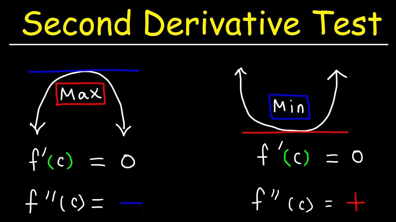
This calculus video tutorial provides a basic introduction into the second derivative test. It explains how to use the second derivative test to identify the presence of a relative maximum or a relative minimum at a critical point. If the second derivative is positive at a critical number – a local minimum is present. If the second derivative is negative at a critical number – a local maximum is present. So to identify the relative extrema, find the first derivative, set it equal to zero and identify the critical numbers. Plug the critical numbers into the second derivative function to determine the concavity of the function to see if its concave up or concave down. If it’s concave up – it’s a relative maximum. If it’s concave down, it’s a relative minimum. You can confirm the results of the second derivative test using the first derivative test with a sign chart on a number line. This video contains plenty of examples and practice problems.
Calculus Video Playlist:
https://www.youtube.com/watch?v=1xATmTI-YY8\u0026t=25s\u0026list=PL0o_zxa4K1BWYThyV4T2Allw6zY0jEumv\u0026index=1
Access to Premium Videos:
https://www.patreon.com/MathScienceTutor
https://www.facebook.com/MathScienceTutoring/
no analytic 2nd derivatives for this method 주제에 대한 자세한 내용은 여기를 참조하세요.
Subject: CCL: Re No analytic 2nd derivatives for this method
If the keyword is absent CalcAll 2nd-derivatives in the first point it is evaluated, and for the subsequent points hessian is not updated. Basis …
Source: www.ccl.net
Date Published: 6/21/2021
View: 4031
What will be the route section for optimization of transition …
I tried with Td(….) whatever you told but the job is terminating after a few second. Its showing ” No analytic 2nd derivatives for this method.”.
Source: www.researchgate.net
Date Published: 4/4/2022
View: 2802
1000. Unable to compute analytic 2nd derivatives. Choose a …
This message appears if you’ve chosen “Analytic 2nd Derivatives” for the Second Derivatives option (see “Knitro Solver Options” in the chapter “Solver …
Source: www.solver.com
Date Published: 8/4/2021
View: 3853
Development of the Analytic Second Derivatives for the …
One route to improve the efficiency is to use fragment-based methods [4], some of which have analytic second derivatives [5,6,7,8,9,10].
Source: link.springer.com
Date Published: 12/4/2021
View: 8943
Analytical second derivatives for excited electronic states …
96, No. 10, 1533-1541. Analytical second derivatives for excited electronic states using the single excitation configuration interaction method: theory and.
Source: www.tandfonline.com
Date Published: 11/6/2022
View: 9162
G09 Keyword: Freq
The keyword Opt=CalcAll requests that analytic second derivatives be done … Applicable only to methods having analytic frequencies but no …
Source: wild.life.nctu.edu.tw
Date Published: 6/10/2022
View: 2485
Freq – Gaussian.com
… frequencies are computed by determining the second derivatives of … method used in determining analytic frequencies is not physically …
Source: gaussian.com
Date Published: 3/30/2021
View: 7884
주제와 관련된 이미지 no analytic 2nd derivatives for this method
주제와 관련된 더 많은 사진을 참조하십시오 Second Derivative Test. 댓글에서 더 많은 관련 이미지를 보거나 필요한 경우 더 많은 관련 기사를 볼 수 있습니다.
주제에 대한 기사 평가 no analytic 2nd derivatives for this method
- Author: The Organic Chemistry Tutor
- Views: 조회수 334,672회
- Likes: 좋아요 4,552개
- Date Published: 2018. 3. 4.
- Video Url link: https://www.youtube.com/watch?v=G8GAsYkZlpE
CCL:G: Subject: CCL: Re No analytic 2nd derivatives for this method
CCL:G: Subject: CCL: Re No analytic 2nd derivatives for this method
From: “Ol Ga”
Subject: CCL:G: Subject: CCL: Re No analytic 2nd derivatives for this method
Date: Sun, 12 Aug 2007 05:36:18 -0400
Sent to CCL by: “Ol Ga” [eurisco1{}pochta.ru] Dear Alvyn Liang! Keyword CalcAll demands calculation 2nd-derivatives in each point for which energy has been calculated. Gaussian does attempt to calculate 2nd-derivatives analytically. But for the given method it appears it is impossible. In this case it is possible to calculate 2nd-derivatives numerically, using a corresponding method of optimization: Link Function L103 Berny optimizations to minima and TS, STQN transition state searches L106 Numerical differentiation of forces/dipoles to obtain polarizability/hyperpolarizability L110 Double numerical differentiation of energies to produce frequencies L111 Double num. diff. of energies to compute polarizabilities and hyperpolarizabilities L113 EF optimization using analytic gradients L114 EF numerical optimization (using only energies)!!!!!!!! If the keyword is absent CalcAll 2nd-derivatives in the first point it is evaluated, and for the subsequent points hessian is not updated. Basis set has no relation to process of optimization and removal + cannot change anything (try attentively still time and you are convinced of this). Send My e-mail for another discussion. Best Regards. ——— Can anyone tell me why I cannot calculate diffuse function in rob3lyp with keyword ‘opt=calcall’.
1000. Unable to compute analytic 2nd derivatives. Choose a different Second Derivatives Option.
This message appears if you’ve chosen “Analytic 2nd Derivatives” for the Second Derivatives option (see “Knitro Solver Options” in the chapter “Solver Options”), but the PSI Interpreter is unable to compute analytic second derivatives for your problem functions. This may be due to use of a nonsmooth function, or a function whose first derivative is nonsmooth, in your objective or constraints. You may be able to proceed by choosing “Analytic 1st Derivatives” or “Finite Differences” for the Second Derivatives option. In Solver SDK Platform, you do this by setting the EngineParam “SecondDerivatives” parameter. But you should also consider changing the formulas in your model to eliminate functions whose second derivatives are not defined.
Development of the Analytic Second Derivatives for the Fragment Molecular Orbital Method
Deglmann P, Furche F, Ahlrichs R (2002) An efficient implementation of second analytical derivatives for density functional methods. Chem Phys Lett 362:511–518
Alexeev Y, Schmidt MW, Windus TL, Gordon MS (2007) A parallel distributed data CPHF algorithm for analytic Hessians. J Comput Chem 28:1685–1694
Pulay P (1969) Ab initio calculation of force constants and equilibrium geometries in polyatomic molecules. Mol Phys 17:197–204
Gordon MS, Fedorov DG, Pruitt SR, Slipchenko LV (2012) Fragmentation methods: a route to accurate calculations on large systems. Chem Rev 112:632–672
Sakai S, Morita S (2005) Ab initio integrated multi-center molecular orbitals method for large cluster systems: Total energy and normal vibration. J Phys Chem A 109:8424–8429
Rahalkar AP, Ganesh V, Gadre SR (2008) Enabling ab initio hessian and frequency calculations of large molecules. J Chem Phys 129:234101
Jose KVJ, Raghavachari K (2015) Evaluation of energy gradients and infrared vibrational spectra through molecules-in-molecules fragment-based approach. J Chem Theory Comput 11(3):950–961
Hua W, Fang T, Li W, Yu JG, Li S (2008) Geometry optimizations and vibrational spectra of large molecules from a generalized energy-based fragmentation approach. J Phys Chem A 112(43):10864–10872
Collins MA (2014) Molecular forces, geometries, and frequencies by systematic molecular fragmentation including embedded charges. J Chem Phys 141:094108
Liu J, Zhang JZH, He X (2016) Fragment quantum chemical approach to geometry optimization and vibrational spectrum calculation of proteins. Phys Chem Chem Phys 18:1864–1875
Cui Q, Karplus M (2000) Molecular properties from combined qm/mm methods. I. Analytical second derivative and vibrational calculations. J Chem Phys 112:1133
Li H, Jensen JH (2002) Partial Hessian vibrational analysis: the localization of the molecular vibrational energy and entropy. Theor Chem Acc 107:211–219
Jensen JH, Li H, Robertson AD, Molina PA (2005) Prediction and rationalization of protein pKa values using QM and QM/MM methods. J Phys Chem A 109:6634–6643
Ghysels A, Woodcock HL III, Larkin JD, Miller BT, Shao Y, Kong J, Neck DV, Speybroeck VV, Waroquier M, Brooks BR (2011) Efficient calculation of QM/MM frequencies with the mobile block Hessian. J Chem Theory Comput 7:496–514
Hafner J, Zheng W (2009) Approximate normal mode analysis based on vibrational subsystem analysis with high accuracy and efficiency. J Chem Phys 130:194111
Ghysels A, Speybroeck VV, Pauwels E, Catak S, Brooks BR, Neck DV, Waroquier M (2010) Comparative study of various normal mode analysis techniques based on partial Hessians. J Comput Chem 31:994–1007
Kitaura K, Ikeo E, Asada T, Nakano T, Uebayasi M (1999) Fragment molecular orbital method: an approximate computational method for large molecules. Chem Phys Lett 313:701–706
Fedorov DG, Kitaura K (2007) Extending the power of quantum chemistry to large systems with the fragment molecular orbital method. J Phys Chem A 111:6904–6914
Fedorov DG, Nagata T, Kitaura K (2012) Exploring chemistry with the fragment molecular orbital method. Phys Chem Chem Phys 14:7562–7577
Tanaka S, Mochizuki Y, Komeiji Y, Okiyama Y, Fukuzawa K (2014) Electron-correlated fragment-molecular-orbital calculations for biomolecular and nano systems. Phys Chem Chem Phys 16:10310–10344
Fedorov DG (2017) The fragment molecular orbital method: theoretical development, implementation in gamess, and applications. CMS WIREs 7:e1322
Fedorov DG, Asada N, Nakanishi I, Kitaura K (2014) The use of many-body expansions and geometry optimizations in fragment-based methods. Acc Chem Res 47:2846–2856
Schmidt MW, Baldridge KK, Boatz JA, Elbert ST, Gordon MS, Jensen JJ, Koseki S, Matsunaga N, Nguyen KA, Su S, Windus TL, Dupuis M, Montgomery JA (1993) General atomic and molecular electronic structure system. J Comput Chem 14:1347–1363
Nakata H, Nagata T, Fedorov DG, Yokojima S, Kitaura K, Nakamura S (2013) Analytic second derivatives of the energy in the fragment molecular orbital method. J Chem Phys 138:164103
Green MC, Nakata H, Fedorov DG, Slipchenko LV (2016) Radical damage in lipids investigated with the fragment molecular orbital method. Chem Phys Lett 651:56–61
Nakata H, Fedorov DG, Yokojima S, Kitaura K, Nakamura S (2014) Efficient vibrational analysis for unrestricted Hartree-Fock based on the fragment molecular orbital method. Chem Phys Lett 603:67–74
Nakata H, Fedorov DG, Zahariev F, Schmidt MW, Kitaura K, Gordon MS, Nakamura S (2015) Analytic second derivative of the energy for density functional theory based on the three-body fragment molecular orbital method. J Chem Phys 142:124101
Nishimoto Y, Fedorov DG, Irle S (2014) Density-functional tight-binding combined with the fragment molecular orbital method. J Chem Theory Comput 10:4801–4812
Nishimoto Y, Nakata H, Fedorov DG, Irle S (2015) Large-scale quantum-mechanical molecular dynamics simulations using density-functional tight-binding combined with the fragment molecular orbital method. J Phys Chem Lett 6:5034–5039
Nakata H, Nishimoto Y, Fedorov DG (2016) Analytic second derivative of the energy for density-functional tight-binding combined with the fragment molecular orbital method. J Chem Phys 145:044113
Nishimoto Y, Fedorov DG (2017) Three-body expansion of the fragment molecular orbital method combined with density-functional tight-binding. J Comput Chem 38:406–418
Nakano T, Kaminuma T, Sato T, Fukuzawa K, Akiyama Y, Uebayasi M, Kitaura K (2002) Fragment molecular orbital method: use of approximate electrostatic potential. Chem Phys Lett 351:475–480
Nagata T, Fedorov DG, Kitaura K (2010) Importance of the hybrid orbital operator derivative term for the energy gradient in the fragment molecular orbital method. Chem Phys Lett 492:302–308
Nakano T, Kaminuma T, Sato T, Akiyama Y, Uebayasi M, Kitaura K (2000) Fragment molecular orbital method: application to polypeptides. Chem Phys Lett 318:614–618
Fedorov DG, Jensen JH, Deka RC, Kitaura K (2008) Covalent bond fragmentation suitable to describe solids in the fragment molecular orbital method. J Phys Chem A 112:11808–11816
Nishimoto Y, Fedorov DG (2018) Adaptive frozen orbital treatment for the fragment molecular orbital method combined with density-functional tight-binding. J Chem Phys 148:064115
Yamaguchi Y, Schaefer HF III, Osamura Y, Goddard J (1994) A new dimension to quantum chemistry: analytical derivative methods in ab initio molecular electronic structure theory. Oxford University Press, New York
Nagata T, Brorsen K, Fedorov DG, Kitaura K, Gordon MS (2011) Fully analytic energy gradient in the fragment molecular orbital method. J Chem Phys 134:124115
Nagata T, Fedorov DG, Kitaura K (2009) Derivatives of the approximated electrostatic potentials in the fragment molecular orbital method. Chem Phys Lett 475:124–131
Nagata T, Fedorov DG, Kitaura K (2012) Analytic gradient for the embedding potential with approximations in the fragment molecular orbital method. Chem Phys Lett 544:87–93
Nakata H, Fedorov DG (2018) Analytic second derivatives for the efficient electrostatic embedding in the fragment molecular orbital method. J Comput Chem 39:2039–2050
Fedorov DG, Alexeev Y, Kitaura K (2011) Geometry optimization of the active site of a large system with the fragment molecular orbital method. J Phys Chem Lett 2:282–288
Fedorov DG, Ishida T, Kitaura K (2005) Multilayer formulation of the fragment molecular orbital method (FMO). J Phys Chem A 109:2638–2646
Aikens CM, Webb SP, Bell RL, Fletcher GD, Schmidt MW, Gordon MS (2003) A derivation of the frozen-orbital unrestricted open-shell and restricted closed-shell second-order perturbation theory analytic gradient expressions. Theor Chem Acc 110:233–253
Handy NC, Schaefer HF III (1984) On the evaluation of analytic energy derivatives for correlated wave functions. J Chem Phys 81:5031–5033
Nagata T, Fedorov DG, Ishimura K, Kitaura K (2011) Analytic energy gradient for second-order Møller-Plesset perturbation theory based on the fragment molecular orbital method. J Chem Phys 135:044110
Fedorov DG, Kitaura K (2004) The importance of three-body terms in the fragment molecular orbital method. J Chem Phys 120:6832–6840
Fedorov DG, Kitaura K (2004) On the accuracy of the 3-body fragment molecular orbital method (FMO) applied to density functional theory. Chem Phys Lett 389:129–134
Nakata H, Fedorov DG, Nagata T, Yokojima S, Ogata K, Kitaura K, Nakamura S (2012) Unrestricted Hartree-Fock based on the fragment molecular orbital method: energy and its analytic gradient. J Chem Phys 137:044110
Komornicki A, McIver JW (1979) An efficient abinitio method for computing infrared and Raman intensities: application to ethylene. J Chem Phys 70(4):2014–2016
Bacskay GB, Saebø S, Taylor PR (1984) On the calculation of dipole moment and polarizability derivatives by the analytical energy gradient method: application to the formaldehyde molecule. Chem Phys 90:215–224
Nakata H, Fedorov DG, Yokojima S, Kitaura K, Nakamura S (2014) Simulations of Raman spectra using the fragment molecular orbital method. J Chem Theory Comput 10(9):3689–3698
Jacob CR, Luber S, Reiher M (2009) Analysis of secondary structure effects on the IR and Raman spectra of polypeptides in terms of localized vibrations. J Phys Chem B 113(18):6558–6573
Weymuth T, Jacob CR, Reiher M (2010) A local-mode model for understanding the dependence of the extended amide III vibrations on protein secondary structure. J Phys Chem B 114:10649–10660
Weymuth T, Haag MP, Kiewisch K, Luber S, Schenk S, Jacob CR, Herrmann C, Neugebauer J, Reiher M (2012) Movipac: vibrational spectroscopy with a robust meta-program for massively parallel standard and inverse calculations. J Comput Chem 33:2186–2198
Nakata H, Fedorov DG, Nagata T, Kitaura K, Nakamura S (2015) Simulations of chemical reactions with the frozen domain formulation of the fragment molecular orbital method. J Chem Theory Comput 11:3053–3064
Albery WJ, Knowles JR (1976) Free-energy profile for the reaction catalyzed by triosephosphate isomerase. Biochemistry 15:5627–5631
Zhang Y, Liu H, Yang W (2000) Free energy calculation on enzyme reactions with an efficient iterative procedure to determine minimum energy paths on a combined ab initio QM/MM potential energy surface. J Chem Phys 112:3483–3492
Ishida T, Fedorov DG, Kitaura K (2006) All electron quantum chemical calculation of the entire enzyme system confirms a collective catalytic device in the chorismate mutase reaction. J Phys Chem B 110:1457–1463
Ito M, Brinck T (2014) Novel approach for identifying key residues in enzymatic reactions: proton abstraction in ketosterbid isomerase. J Phys Chem B 118:13050–13058
Jensen JH, Willemos M, Winther JR, De Vico L (2014) In silico prediction of mutant HIV-1 proteases cleaving a target sequence. PLoS ONE 9:e95833
Fedorov DG, Kitaura K (2007) Pair interaction energy decomposition analysis. J Comput Chem 28:222–237
Ahmed Z, Beta IA, Mikhonin AV, Asher SA (2005) UV resonance Raman thermal unfolding study of Trp-cage shows that it is not a simple two-state miniprotein. J Am Chem Soc 127:10943–10950
Scott AP, Radom L (1996) Harmonic vibrational frequencies: an evaluation of Hartree-Fock, Møller-Plesset, quadratic configuration interaction, density functional theory, and semiempirical scale factors. J Phys Chem 100:16502–16513
G09 Keyword: Freq
Freq
DESCRIPTION
This calculation type keyword computes force constants and the resulting vibrational frequencies. Intensities are also computed. By default, the force constants are determined analytically if possible (for AM1, PM3, PM3MM, PM6, PDDG, RHF, UHF, MP2, CIS, all DFT methods and CASSCF), by single numerical differentiation for methods for which only first derivatives are available (MP3, MP4(SDQ), CID, CISD, CCD, CCSD, BD and QCISD), and by double numerical differentiation for those methods for which only energies are available.
Vibrational frequencies are computed by determining the second derivatives of the energy with respect to the Cartesian nuclear coordinates and then transforming to mass-weighted coordinates. This transformation is only valid at a stationary point! Thus, it is meaningless to compute frequencies at any geometry other than a stationary point for the method used for frequency determination.
For example, computing 6-311G(d) frequencies at a 6-31G(d) optimized geometry produces meaningless results. It is also incorrect to compute frequencies for a correlated method using frozen core at a structure optimized with all electrons correlated, or vice-versa. The recommended practice is to compute frequencies following a previous geometry optimization using the same method. This may be accomplished automatically by specifying both Opt and Freq within the route section for a job.
Note also that the CPHF (coupled perturbed SCF) method used in determining analytic frequencies is not physically meaningful if a lower energy wavefunction of the same spin multiplicity exists. Use the Stable keyword to test the stability of Hartree-Fock and DFT wavefunctions.
FREQUENCY CALCULATION VARIATIONS
Additional related properties may also be computed during frequency calculations, including the following:
When frequencies are done analytically, polarizabilities are also computed automatically; when numerical differentiation is required (or requested with Freq=Numer ), polarizabilities must be explicitly requested using the Polar keyword (e.g., CCSD Freq Polar ).
The VCD option may be used to compute the vibrational circular dichroism (VCD) intensities in addition to the normal frequency analysis at the Hartree-Fock and DFT levels [Cheeseman96a] .
The ROA option computes analytic Raman optical activity intensities [Helgaker94, Dukor00, Ruud02a, Barron04, Thorvaldsen08, Cheeseman11a] .
Pre-resonance Raman intensities may be computed by specifying one of the Raman options, and also including CPHF=RdFreq within the route and specifying the desired frequency in the input file (see the examples for additional information).
Frequency-dependent polarizabilities and hyperpolarizabilities may be computed by including CPHF=RdFreq within the route (subject to their usual availability restrictions).
Vibrational-rotational coupling can be computed using Freq=VibRot [Califano76, Miller80, Papousek82, Clabo88, Page88, Adamo90, Miller90, Page90, Barone03] . Numerical differentiation can also be performed along modes to compute zero-point energies, anharmonic frequencies [Califano76, Miller80, Papousek82, Clabo88, Page88, Miller90, Page90, Barone04, Barone05] , and anharmonic vibrational-rotational couplings if Anharmonic is also specified [Adamo90, Barone94, Minichino94, Barone95, Barone03] . This option is only available for methods with analytic second derivatives: Hartree-Fock, DFT, CIS and MP2. Full anharmonic IR intensities are computed [Bloino12] . The DCPT2 [Kuhler96, Bloino12a] and HDCPT2 [Bloino12a] methods support resonance-free computations of anharmonic frequencies and partition functions. Vibronic computations include ECD [Barone12] .
There are several options for performing an analysis for an electronic excitation using the Franck-Condon and/or Herzberg-Teller methods (see below).
The keyword Opt=CalcAll requests that analytic second derivatives be done at every point in a geometry optimization. Once the requested optimization has completed all the information necessary for a frequency analysis is available. Therefore, the frequency analysis is performed and the results of the calculation are archived as a frequency job.
INPUT FOR SELECTING NORMAL MODES
These sections specify the format of the input sections for the SelectNormalModes , SelectAnharmonicModes and SelectFranckCondonModes options. The modes to select are specified in a separate blank-line terminated input section. The initial mode list is always empty.
Integers and integer ranges without a keyword are interpreted as mode numbers, although the [ not ] mode keywords may be used. The keywords atoms and notatoms can be used to define an atom list whose modes should be included/excluded (respectively). Atoms can also be specified by ONIOM layer via the [ not ] layer keywords, which accept these values: real for the real system, model for the model system in a 2-layer ONIOM, middle for the middle layer in a 3-layer ONIOM, and small for the model layer of a 3-layer ONIOM. Atoms may be similarly included/excluded by residue with residue and notresidue , which accept lists of residue names or numbers. Both keyword sets function as shorthand forms for atom lists.
Here are some examples:
2-5 Includes modes 2 through 5. atoms=O Includes modes involving oxygen atoms. 1-20 atoms=Fe Includes modes 1 through 20 and any modes involving iron atoms. layer=real notatoms=H Includes modes for heavy atoms in low layer (subject to default threshold).
OPTIONS REQUESTING SPECIFIC PROPERTIES/ANALYSES
Raman
Compute Raman intensities in addition to IR intensities. This is the default for Hartree-Fock. It may be specified for DFT and MP2 calculations. For MP2, Raman intensities are produced by numerical differentiation of dipole derivatives with respect to the electric field (equivalent to NRaman ).
NRaman
Compute polarizability derivatives by numerically differentiating the analytic dipole derivatives with respect to an electric field. This is the default for MP2=Raman .
NNRaman
Compute polarizability derivatives by numerically differentiating the analytic polarizability with respect to nuclear coordinates.
NoRaman
Skips the extra steps required to compute the Raman intensities during Hartree-Fock analytic frequency calculations, saving 10-30% in CPU time.
VCD
Compute the vibrational circular dichroism (VCD) intensities in addition to the normal frequency analysis. This option is valid for Hartree-Fock and DFT methods. This option also computes optical rotations (see Polar=OptRot ).
ROA
Compute dynamic analytic Raman optical activity intensities using GIAOs [Cheeseman11a] . This procedure requires one or more incident light frequencies to be supplied in the input to be used in the electromagnetic perturbations ( CPHF=RdFreq is the default with Freq=ROA ). This option is valid for Hartree-Fock and DFT methods. NNROA says to use the numerical ROA method from Gaussian 03; this is useful only for reproducing the results of prior calculations.
VibRot
Analyze vibrational-rotational coupling.
Anharmonic
Do numerical differentiation along modes to compute zero-point energies, anharmonic frequencies, and anharmonic vibrational-rotational couplings if VibRot is also specified. This option is only available for methods with analytic second derivatives: Hartree-Fock, DFT, CIS and MP2. This output includes IR intensities.
ReadAnharm
Read an input section with additional parameters for the vibrational-rotational coupling and/or anharmonic vibrational analysis ( VibRot or Anharmonic options). Available input options are documented below following the examples.
SelectAnharmonicModes
Read an input section selecting which modes are used for differentiation in anharmonic analysis. The format of this input section is discussed above. SelAnharmonicModes is a synonym for this option.
Projected
For a point on a mass-weighted reaction path (IRC), compute the projected frequencies for vibrations perpendicular to the path. For the projection, the gradient is used to compute the tangent to the path. Note that this computation is very sensitive to the accuracy of the structure and the path [Baboul97] . Accordingly, the geometry should be specified to at least 5 significant digits. This computation is not meaningful at a minimum.
HinderedRotor
Requests the identification of internal rotation modes during the harmonic vibrational analysis [McClurg97, Ayala98, McClurg99] . If any modes are identified as internal rotation, hindered or free, the thermodynamic functions are corrected. The identification of the rotating groups is made possible by the use of redundant internal coordinates. Because some structures, such as transition states, may have a specific bonding pattern not automatically recognized, the set of redundant internal coordinates may need to be altered via the Geom=Modify keyword. Rotations involving metals require additional input via the ReadHinderedRotor option (see below).
If the force constants are available on a previously generated checkpoint file, additional vibrational/internal rotation analyses may be performed by specifying Freq=(ReadFC, HinderedRotor) . Since Opt=CalcAll automatically performs a vibrational analysis on the optimized structure, Opt=(CalcAll, HinderedRotor) may also be used.
ReadHinderedRotor
Causes an additional input section to be read containing the rotational barrier cutoff height (in kcal/mol) and optionally the periodicity, symmetry number and multiplicity for rotational modes. Rotations with barrier heights larger than the cutoff value will be automatically frozen. If the periodicity value is negative, then the corresponding rotor is also frozen. You must provide the periodicity, symmetry and spin multiplicity for all rotatable bonds contain metals. The input section is terminated with a blank line, and has the following format:
VMax-value Atom1 Atom2 periodicity symmetry spin Repeated as necessary. …
ELECTRONIC EXCITATION ANALYSIS OPTIONS
The following options perform an analysis for an electronic excitation using the corresponding method; these jobs use vibrational analysis calculations for the ground state and the excited state to compute the amplitudes for electronic transitions between the two states. The vibrational information for the ground state is taken from the current job ( Freq or Freq=ReadFC ), and the vibrational information for the excited state is taken from a checkpoint file, whose name is provided in a separate input section (enclose the path in quotes if it contains internal spaces). The latter will be from a CI-Singles or TD-DFT Freq=SaveNormalModes calculation.
The ReadFCHT option can be added to cause additional input to be read to control these calculations (see below), and the SelFCModes option can be used to select the modes involved. In the latter case, the excited state checkpoint file would typically have been generated with Freq=(SelectNormalModes, SaveNormalModes) with the same modes selected.
If CIS frequencies are to be used with the Herzberg-Teller or Franck-Condon-Herzberg-Teller analysis, the CIS frequencies must be done numerically ( Freq=Numer rather than Freq ). This is because the transition dipole derivatives are not computed during the analytic force constant evaluation. The corresponding HF frequency calculation on the ground state, which is also required, can be done analytically as usual.
FranckCondon
Use the Franck-Condon method [Sharp64, Doktorov77, Kupka86, Zhixing89, Berger97, Peluso97, Berger98, Borrelli03, Weber03, Coutsias04, Dierksen04, Lami04, Dierksen04a, Dierksen05, Liang05, Jankowiak07, Santoro07, Santoro07a, Barone09] (the implementation is described in [Santoro07, Santoro07a, Santoro08, Barone09] ). FC is a synonym for this option. Transitions for ionizations can be analyzed instead of excitations. In this case, the molecule specification corresponds to the neutral form, and the additional checkpoint file named in the input section corresponds to the cation.
HerzbergTeller
Use the Herzberg-Teller method [Herzberg33, Sharp64, Small71, Orlandi73, Lin74, Santoro08] (the implementation is described in [Santoro08] ). HT is a synonym for this option.
FCHT
Use the Franck-Condon-Herzberg-Teller method [Santoro08] .
Emission
Indicates that emission rather than absorption should be simulated for a Franck-Condon and/or Herzberg-Teller analysis. In this case, within the computation the initial state is the excited state, and the final state is the ground state (although the sources of frequency data for the ground and excited state are as described above: current job=ground state, second checkpoint file=excited state).
ReadFCHT
Read an input section containing parameters for the calculation. Available input options are documented below following the examples. This input section precedes that for ReadAnharmon if both are present.
SelectFranckCondonModes
Read an input section selecting which modes are used for differentiation in Franck-Condon analysis. The format of this input section is discussed above. This input section precedes that for SelectAnharmonicModes if both are present, and the modes are specified in the usual Gaussian order (increasing), not the order displayed in the anharmonic output. SelFCModes is a synonym for this option.
NORMAL MODE RELATED OPTIONS
HPModes
Include the high precision format (to five figures) vibrational frequency eigenvectors in the frequency output in addition to the normal three-figure output.
InternalModes
Print modes as displacements in redundant internal coordinates. IntModes is a synonym for this option.
SaveNormalModes
Save all modes in the checkpoint file. SaveNM is a synonym for this option. NoSaveNormalModes , or NoSaveNM , is the default.
ReadNormalModes
Read saved modes from the checkpoint file. ReadNM is a synonym for this option. NoReadNormalModes , or NoReadNM , is the default.
SelectNormalModes
Read input selecting the particular modes to display. SelectNM is a synonym for this option. NoSelectNormalModes , or NoSelectNM , is the default. AllModes says to include all modes in the output. The format of this input section is discussed above. Note that this option does not affect the functioning of SaveNormalModes , which always saves all modes in the checkpoint file.
SortModes
Sort modes by ONIOM layer in the output.
ModelModes
Display only modes involving the smallest model system in an ONIOM calculation.
MiddleModes
Display only modes involving the two model systems in a 3-layer ONIOM.
PrintFrozenAtoms
By default, the zero displacements for frozen atoms are not printed in the mode output. This option requests that all atoms be listed.
NoPrintNM
Used to suppress printing of the normal mode components during a frequency calculation. The frequencies and intensities are still reported for each mode.
MOLECULE SPECIFICATION MODIFICATION OPTIONS
ModRedundant
Read-in modifications to redundant internal coordinates (i.e., for use with InternalModes ). Note that the same coordinates are used for both optimization and mode analysis in an Opt Freq , for which this is the same as Opt=ModRedundant . See the discussion of the Opt keyword for details on the input format.
ReadIsotopes
This option allows you to specify alternatives to the default temperature, pressure, frequency scale factor and/or isotopes—298.15 K, 1 atmosphere, no scaling, and the most abundant isotopes (respectively). It is useful when you want to rerun an analysis using different parameters from the data in a checkpoint file.
Be aware, however, that all of these can be specified in the route section ( Temperature , Pressure and Scale keywords) and molecule specification ( Iso= parameter), as in this example:
#T Method /6-31G(d) JobType Temperature=300.0 … … 0 1 C(Iso=13) …
ReadIsotopes
temp pressure [ scale ] Values must be real numbers. isotope mass for atom 1 isotope mass for atom 2 … isotope mass for atom n
where temp , pressure , and scale are the desired temperature, pressure, and an optional scale factor for frequency data when used for thermochemical analysis (the default is unscaled). The remaining lines hold the isotope masses for the various atoms in the molecule, arranged in the same order as they appeared in the molecule specification section. If integers are used to specify the atomic masses, the program will automatically use the corresponding actual exact isotopic mass (e.g., 18 specifies 18O, and Gaussian uses the value 17.99916).
ALGORITHM AND PROCEDURE RELATED OPTIONS
Analytic
This specifies that the second derivatives of the energy are to be computed analytically. This option is available only for RHF, UHF, CIS, CASSCF, MP2, and all DFT methods, and it is the default for those cases.
Numerical
This requests that the second derivatives of the energy are to be computed numerically using analytically calculated first derivatives. It can be used with any method for which gradients are available and is the default for those for which gradients but not second derivatives are available. Freq=Numer can be combined with Polar=Numer in one job step.
DoubleNumer
This requests double numerical differentiation of energies to produce force constants. It is the default and only choice for those methods for which no analytic derivatives are available. EnOnly is a synonym for DoubleNumer .
Cubic
Requests numerical differentiation of analytic second derivatives to produce third derivatives. Applicable only to methods having analytic frequencies but no analytic third derivatives.
Step= N
Specifies the step-size for numerical differentiation to be 0.0001* N (in Angstoms unless Units=Bohr has been specified). If Freq=Numer and Polar=Numer are combined, N also specifies the step-size in the electric field. The default is 0.001 Å for Hartree-Fock and correlated Freq=Numer , 0.005 Å for GVB and CASSCF Freq=Numer , and 0.01 Å for Freq=EnOnly . For Freq=Anharmonic or Freq=VibRot , the default is 0.025 Å.
Restart
This option restarts a numerical frequency calculation after the last completed geometry. A failed numerical frequency job may be restarted from its checkpoint file by simply repeating the route section of the original job, adding the Restart option to the Freq=Numer keyword/option. No other input is required.
Analytic frequencies can be restarted with the Restart keyword provided that the read-write file was named and saved from the failed job. See the description of that keyword for more information and an example.
DiagFull
Diagonalize the full ( 3N atoms )2 force constant matrix—including the translation and rotational degrees of freedom—and report the lowest frequencies to test the numerical stability of the frequency calculation. This precedes the normal frequency analysis where these modes are projected out. Its output reports the lowest 9 modes, the upper 3 of which correspond to the 3 smallest modes in the regular frequency analysis. Under ideal conditions, the lowest 6 modes reported by this analysis will be very small in magnitude. When they are significantly non-zero, it indicates that the calculation is not perfectly converged/numerically stable. This may indicate that translations and rotations are important modes for this system, that a better integration grid is needed, that the geometry is not converged, etc. The system should be studied further in order to obtain accurate frequencies. See the examples section below for the output from this option.
DiagFull is the default; NoDiagFull says to skip this analysis.
ReadFC
Requests that the force constants from a previous frequency calculation be read from the checkpoint file, and the mode and thermochemical analysis be repeated, presumably using a different temperature, pressure, or isotopes, at minimal computational cost. Note that since the basis set is read from the checkpoint file, no general basis should be input. If the Raman option was specified in the previous job, then do not specify it again when using this option.
TwoPoint
When computing numerical derivatives, make two displacements in each coordinate. This is the default. FourPoint will make four displacements but only works with Link 106 ( Freq=Numer ). Not valid with Freq=DoubleNumer .
NFreq= N
Requests that the lowest N frequencies be solved for using Davidson diagonalization. At present, this option is only available for ONIOM(QM:MM) model chemistries.
AVAILABILITY
Analytic frequencies are available for the AM1, PM3, PM3MM, PM6, PDDG, DFTB, DFTBA, HF, DFT, MP2, CIS and CASSCF methods. Numerical frequencies are available for MP3, MP4(SDQ), CID, CISD, CCD, CCSD and QCISD. Raman is available for the HF, DFT and MP2 methods. VCD and ROA are available for HF and DFT methods. Anharmonic is available for HF, DFT, MP2 and CIS methods. Freq and NMR can now both be on the same route for HF and DFT.
RELATED KEYWORDS
Polar , Opt , Stable , NMR .
EXAMPLES
Frequency Output. The basic components of the output from a frequency calculation are discussed in detail in chapter 4 of Exploring Chemistry with Electronic Structure Methods [Foresman96b] .
New Gaussian users are often surprised to see that the final part frequency calculation output that looks that of a geometry optimization at the beginning of a frequency job:
GradGradGradGradGradGradGradGradGradGradGradGradGradGradGrad Berny optimization. Initialization pass.
Link 103, which performs geometry optimizations, is executed at the beginning and end of all frequency calculations. This is done so that the quadratic optimization step can be computed using the correct second derivatives. Occasionally an optimization will complete according to the normal criterion using the approximate Hessian matrix, but the step size is actually larger than the convergence criterion when the correct second derivatives are used. The next step is printed at the end of a frequency calculation so that such problems can be identified. If you think this concern is applicable, use Opt=CalcAll instead of Freq in the route section of the job, which will complete the optimization if the geometry is determined not to have fully converged (usually, given the full second derivative matrix near a stationary point, only one additional optimization step is needed), and will automatically perform a frequency analysis at the final structure.
Specifying #P in the route section produces some additional output for frequency calculations. Of most importance are the polarizability and hyperpolarizability tensors (they still may be found in the archive entry in normal print-level jobs). They are presented in lower triangular and lower tetrahedral order, respectively (i.e., α xx , α xy , α yy , α xz , α yz , α zz and β xxx , β xxy , β xyy , β yyy , β xxz , β xyz , β yyz , β xzz , β yzz , β zzz ), in the standard orientation:
Dipole = 2.37312183D-16 -6.66133815D-16 -9.39281319D-01 Polarizability= 7.83427191D-01 1.60008472D-15 6.80285860D+00 -3.11369582D-17 2.72397709D-16 3.62729494D+00 HyperPolar = 3.08796953D-16 -6.27350412D-14 4.17080415D-16 5.55019858D-14 -7.26773439D-01 -1.09052038D-14 -2.07727337D+01 4.49920497D-16 -1.40402516D-13 -1.10991697D+01
#P also produces a bar-graph of the simulated spectra for small cases.
Thermochemistry analysis follows the frequency and normal mode data:
Zero-point correction= .023261 (Hartree/Particle) Thermal correction to Energy= .026094 Thermal correction to Enthalpy= .027038 Thermal correction to Gibbs Free Energy= .052698 Sum of electronic and zero-point Energies=-527.492585 E 0 =E elec +ZPE Sum of electronic and thermal Energies= -527.489751 E= E 0 + E vib + E rot +E trans Sum of electronic and thermal Enthalpies=-527.488807 H=E+RT Sum of electronic and thermal Free Energies=-527.463147 G=H-TS
The raw zero-point energy correction and the thermal corrections to the total energy, enthalpy, and Gibbs free energy (all of which include the zero-point energy) are listed, followed by the corresponding corrected energy. The analysis uses the standard expressions for an ideal gas in the canonical ensemble. Details can be found in McQuarrie [McQuarrie73] and other standard statistical mechanics texts. In the output, the various quantities are labeled as follows:
E (Thermal) Contributions to the thermal energy correction CV Constant volume molar heat capacity S Entropy Q Partition function
The thermochemistry analysis treats all modes other than the free rotations and translations as harmonic vibrations. For molecules having hindered internal rotations, this can produce slight errors in the energy and heat capacity at room temperatures and can have a significant effect on the entropy. The contributions of any very low frequency vibrational modes are listed separately so that their harmonic contributions can be subtracted from the totals and their correctly computed contributions included should they be group rotations and high accuracy is required. Expressions for hindered rotational contributions to these terms can be found in Benson [Benson68] . The partition functions are also computed, with both the bottom of the vibrational well and the lowest (zero-point) vibrational state as reference.
Pre-resonance Raman. This calculation type is requested with one of the Raman options in combination with CPHF=RdFreq . The frequency specified for the latter should be chosen as follows:
Determine the difference in frequency between the peak of interest in the Raman spectrum and the incident light used in the experiment.
Perform a TD calculation using a DFT method in order to determine the predicted location of the same peak.
calculation using a DFT method in order to determine the predicted location of the same peak. Specify a frequency for CPHF=RdFreq which is shifted from the predicted peak by the same amount as the incident light differs from the observed peak.
Pre-resonance Raman results are reported as additional rows within the normal frequency tables:
Harmonic frequencies (cm**-1), IR intensities (KM/Mole), Raman scattering activities (A**4/AMU), depolarization ratios for plane and unpolarized incident light, reduced masses (AMU), force constants (mDyne/A), and normal coordinates: 1 B1 Frequencies — 1315.8011 Red. masses — 1.3435 Frc consts — 1.3704 IR Inten — 7.6649 Raman Activ — 0.0260 Depolar (P) — 0.7500 Depolar (U) — 0.8571 RamAct Fr= 1– 0.0260 Additional output lines begin here. Dep-P Fr= 1– 0.7500 Dep-U Fr= 1– 0.8571 RamAct Fr= 2– 0.0023 Dep-P Fr= 2– 0.7500 Dep-U Fr= 2– 0.8571
Vibration-Rotation Coupling Output. If the VibRot option is specified, then the harmonic vibrational-rotational analysis appears immediately after the normal thermochemistry analysis in the output, introduced by this header:
Vibro-Rotational Analysis at the Harmonic level
If anharmonic analysis is requested as well (i.e., VibRot and Anharmonic are both specified), then the anharmonic vibrational-rotational analysis results follow the harmonic ones, introduced by the following header:
2nd order Perturbative Anharmonic Analysis
Anharmonic Frequency Calculations. Freq=Anharmonic jobs produce additional output following the normal frequency output. (It follows the vibrational-rotational coupling output if this was specified as well.) We will briefly consider the most important items.
The output displays the equilibrium geometry (i.e., the minimum on the potential energy surface), followed by the anharmonic vibrationally averaged structure at 0 K:
Internal coordinates for the Equilibrium structure (Se) Interatomic distances: 1 2 3 4 1 C 0.000000 2 O 1.206908 0.000000 3 H 1.083243 2.008999 0.000000 4 H 1.083243 2.008999 1.826598 0.000000 Interatomic angles: O2-C1-H3=122.5294 O2-C1-H4=122.5294 H3-C1-H4=114.9412 O2-H3-H4= 62.9605 Dihedral angles: H4-C1-H3-O2= 180. Internal coordinates for the vibr.aver. structure at 0K (Sz) Interatomic distances: 1 2 3 4 1 C 0.000000 2 O 1.210431 0.000000 3 H 1.097064 2.024452 0.000000 4 H 1.097064 2.024452 1.849067 0.000000 Interatomic angles: O2-C1-H3=122.57 O2-C1-H4=122.57 H3-C1-H4=114.8601 O2-H4-H3= 62.8267 Dihedral angles: H4-C1-H3-O2= 180.
Note that the bond lengths are slightly longer in the latter structure. The anharmonic zero point energy is given shortly thereafter in the output, preceded by its component terms:
ZPEharm = 6359.86859 cm-1 = 18.184 Kcal/mol = 76.081 Kj/mol ZPEfund = 6135.92666 cm-1 = 17.543 Kcal/mol = 73.402 KJ/mol ZPEaver = 6247.89762 cm-1 = 17.864 Kcal/mol = 74.741 KJ/mol -1/4sumXii = 22.67024 cm-1 = 0.065 Kcal/mol = 0.271 KJ/mol x0 = -6.63071 cm-1 = -0.019 Kcal/mol = -0.079 KJ/mol ZPEtot = 6263.93715 cm-1 = 17.909 Kcal/mol = 74.933 KJ/mol ZPEtot/ZPEharm = 0.98492 ZPEfund/ZPEharm= 0.96479
The anharmonic frequencies themselves appear just a bit later in this table, in the column labeled E(anharm) :
Vibrational Energies and Rotational Constants (cm-1) Mode(Quanta) E(harm) E(anharm) Aa(z) Ba(x) Ca(y) Equilibrium Geometry 10.026637 1.293823 1.145922 Ground State 6359.869 6263.937 9.905085 1.288586 1.136128 Fundamental Bands (DE w.r.t. Ground State) 1(1) 3162.302 2990.777 9.727534 1.287879 1.133639 2(1) 1915.637 1884.683 9.913583 1.284564 1.128397 3(1) 1692.660 1657.100 9.955741 1.294044 1.133257 4(1) 1337.296 1315.965 6.861429 1.277085 1.137163 5(1) 3233.358 3068.112 9.809451 1.286693 1.134405 6(1) 1378.483 1355.216 12.919667 1.290780 1.130316
The harmonic frequencies are also listed for convenience.
Examining Low Lying Frequencies. The output from the full force constant matrix diagonalization (the default Freq=DiagFull ), in which the rotational and translational degrees of freedom are retained, appears as following in the output:
Low frequencies — -19.9673 -0.0011 -0.0010 0.0010 14.2959 25.6133 Low frequencies — 385.4672 988.9028 1083.0692
This output is from an Opt Freq calculation on methanol. Following that are essentially 0, the lowest modes (ignoring sign) are located at around 14, 19 and 25 wavenumbers. If we rerun the calculation using tight optimization criteria and a larger integration grid ( Opt=Tight Int=UltraFine ), the lowest modes become:
Low frequencies — -7.4956 -5.4813 -2.6908 0.0003 0.0007 0.0011 Low frequencies — 380.1699 988.1436 1081.9083
The low-lying modes are now quite small, and the lowest frequencies have moved slightly as a result.
This analysis is especially important for molecular systems having frequencies at small wavenumbers. For example, if the lowest reported frequency is around 30 and there is a low lying mode around 25 as above, then the former value is in considerable doubt (as is whether the molecular structure is even a minimum).
Rerunning a Frequency Calculation with Different Thermochemistry Parameters. The following two-step job contains an initial frequency calculation followed by a second thermochemistry analysis using a different temperature, pressure, and selection of isotopes:
%Chk=freq # HF/6-31G(d,p) Freq Test Frequencies at STP molecule specification -Link1- %Chk=freq %NoSave # HF/6-31G(d,p) Freq(ReadIso,ReadFC) Geom=Check Test Repeat at 300 K 0,1 300.0 1.0 16 2 3 …
Note also that the freqchk utility may be used to rerun the thermochemical analysis from the frequency data stored in a Gaussian checkpoint file.
ADDITIONAL INPUT FOR FREQ=READANHARM
This input is read in a separate section. Its format changed with revision D.01. The following table gives the equivalents for the older keyword forms:
Old Keyword New Keyword DaDeMin Resonances=DaDeMin DelFre Resonances=DFreqDD DelVPT Resonances=DPT2Var EnerInp InpDEner Fermi Property=Fermi InDerAJ DataSrc=InDerAJ InDerAU DataSrc=InDerAU InDerGau DataSrc=InDerGau InDerRed DataSrc=InDerRed InFreq DataAdd=Freq InGauDer DataSrc=InGauDer NoCor DataMod=NoCor NoReord DataSrc=NMOrder=DescNoIrrep; Print=NMOrder=DescNoIrrep Reduced DataSrc=Reduced Reord DataSrc=NMOrder=Desc; Print=NMOrder=Desc ScHarm DataMod=ScHarm TolCor Tolerances=Coriolis TolDE3 Tolerances=Cubic TolDE4 Tolerances=Quartic TolGra Tolerances=Gradient TolHes Tolerances=Hessian TolIne Tolerances=Inertia
Output Control
Print=items
Control the printing of data. Items can include:
Verbosity= n : Select the level of verbosity (default=0).
: Select the level of verbosity (default=0). NMOrder= keyword : Selects the order in which normal modes are printed. Keyword is one of: DescByIrrep (group by symmetry irreducible representation and use descending order within each group, i.e. spectroscopic order. This is the default with symmetry), DescNoIrrep (do not group by symmetry and use descending order; this is the default if symmetry is deactivated); AscByIrrep (group by symmetry irreducible representation and use ascending order within each group); AscNoIrrep (do not group by symmetry and use ascending order). Desc is synonymous with DescByIrrep , and Asc is synonymous with AscByIrrep .
: Selects the order in which normal modes are printed. is one of: (group by symmetry irreducible representation and use descending order within each group, i.e. spectroscopic order. This is the default with symmetry), (do not group by symmetry and use descending order; this is the default if symmetry is deactivated); (group by symmetry irreducible representation and use ascending order within each group); (do not group by symmetry and use ascending order). is synonymous with , and is synonymous with . ITop= keyword : Selects the representation used for the vibro-rotational terms. By default, it is defined automatically by Gaussian from the principal moments of inertia. Available keywords are: Ir : Representation Ir: I z < I x < I y IIr : Representation IIr: I y < I z < I x IIIr : Representation IIIr: I x < I y < I z IIIl : Representation IIIl: I y < I x < I z : Selects the representation used for the vibro-rotational terms. By default, it is defined automatically by Gaussian from the principal moments of inertia. Available keywords are: Data Treatment DataSrc=keyword Select the main source of data, via one of the following keywords: Calc : Use data from the current job. This is the default. : Use data from the current job. This is the default. Chk [ = Rebuild ]: Use anharmonic data from the checkpoint file. If the Rebuild option is specified, then rebuild anharmonic data from various RWF of the checkpoint file. [ ]: Use anharmonic data from the checkpoint file. If the option is specified, then rebuild anharmonic data from various RWF of the checkpoint file. InDerAU : Use data from the input stream in atomic units : Use data from the input stream in atomic units InDerAJ : Use data from the input stream in attoJoules : Use data from the input stream in attoJoules InDerRed : Use data from the input stream in reduced form : Use data from the input stream in reduced form Reduced : Use data from the input stream in reduced form : Use data from the input stream in reduced form InDerGau : Use data from the input stream with the layout of the Gaussian output : Use data from the input stream with the layout of the Gaussian output InGauDer : Use data from the input stream with the layout of the Gaussian output : Use data from the input stream with the layout of the Gaussian output NMOrder= keyword : Selects the order in which normal modes are stored. Keyword is one of: Print (use the same order than that selected for printing see Print=NMOrder= keyword ); DescByIrrep (group by symmetry irreducible representation and use descending order within each group, i.e. spectroscopic order; this is the default with symmetry); DescNoIrrep (do not group by symmetry and use descending order; this is the default if symmetry is deactivated); AscByIrrep (group by symmetry irreducible representation and use ascending order within each group); AscNoIrrep (do not group by symmetry and use ascending order). Desc is synonymous with DescByIrrep , and Asc is synonymous with AscByIrrep . DataAdd=Freq Replace harmonic frequencies with values given in input stream (in cm−1). DataMod=items Modify input data with an automatic or semi-automatic procedure. Items can include: ScHarm= f : Scales harmonic frequencies with a constant scaling factor. The default is 1.0. : Scales harmonic frequencies with a constant scaling factor. The default is 1.0. NoCor : Discards Coriolis couplings in calculations : Discards Coriolis couplings in calculations DerOrder= n : Selects the derivative orders to keep. For example, DerOrder=123 discards all quartic force constants. The default is 1234. : Selects the derivative orders to keep. For example, discards all quartic force constants. The default is 1234. DerIndex= n : Sets the maximum number of independent indexes in a derivative. For example, DerIndex=2 keeps k iij but discards k ijk . The default is 4 : Sets the maximum number of independent indexes in a derivative. For example, keeps k but discards k . The default is 4 SkipPT2= keyword : Selectively removes some derivatives. The keyword is one of Modes (cancels the derivatives with respect to at least one of the normal modes given in the input stream), OptModes (sames as Modes but forces Gaussian to read an option line before the list of normal modes) or Constants (cancels the derivatives based on the indexes given in the input stream. E.g., 4 5 6 makes Gaussian reset k 456 ). A single option line in the input is available with DataMod=SkipPT2=OptModes (see below for placement in the Gaussian input file). The available options are: MinInd= n : Controls the minimum number of times a selected normal mode must appear to discard the derivative. E.g., MinInd=2 means that k ijk is kept, but k iij and k iii are removed. The default is 1. EnOrd= n : Controls the energy derivative orders to discard. By default, the reset is done on all energy derivatives. E.g., EnOrd=14 says to only remove the first and fourth energy derivatives and to keep the second and third energy derivatives. The default is 1234. : Selectively removes some derivatives. The keyword is one of (cancels the derivatives with respect to at least one of the normal modes given in the input stream), (sames as but forces Gaussian to read an option line before the list of normal modes) or (cancels the derivatives based on the indexes given in the input stream. E.g., 4 5 6 makes Gaussian reset k ). A single option line in the input is available with (see below for placement in the Gaussian input file). The available options are: Tolerances=items Modify the tolerance threshold to include/discard constants. Items are: Gradient= f : Threshold for the energy first derivatives (default: 3.7074 × 10 −3 ). : Threshold for the energy first derivatives (default: 3.7074 × 10 ). Hessian= f : Threshold for the energy second derivatives (default: 3.7074 × 10 −5 ). : Threshold for the energy second derivatives (default: 3.7074 × 10 ). Cubic= f : Threshold for the energy third derivatives (default: 3.7074 × 10 −5 ). : Threshold for the energy third derivatives (default: 3.7074 × 10 ). Quartic= f : Threshold for the energy fourth derivatives (default: 3.7074 × 10 −5 ). : Threshold for the energy fourth derivatives (default: 3.7074 × 10 ). Coriolis= f : Threshold for the Coriolis couplings (default: 1.0 × 10 −3 ). : Threshold for the Coriolis couplings (default: 1.0 × 10 ). Inertia= f : Threshold for the principal moments of inertia (default: 1.0 × 10⁻⁴ amu·Å2). Reduced-Dimensionality Schemes RedDim=items Controls the selective treatment of a part of the complete system. Items are: Inactive= n : Read modes in the input stream and sets them to be inactive. : Read modes in the input stream and sets them to be inactive. MinFreqIn= f : Sets the normal modes with a frequency above MinFreqIn to be inactive (default: infinity). Only valid if MaxFreqIn > MinFreqIn . If MaxFreqIn is not set by the user, then MinFreqIn automatically sets MaxFreqIn to infinity.
: Sets the normal modes with a frequency above MinFreqIn to be inactive (default: infinity). Only valid if > . If is not set by the user, then automatically sets to infinity. MaxFreqIn= f : Sets the normal modes with a frequency lower than MaxFreqIn to be inactive (default: 0.0). Only valid if MaxFreqIn > MinFreqIn . If MinFreqIn is not set by the user, then MaxFreqIn automatically sets MinFreqIn to 0.0.
Second-order Vibrational Perturbation Theory (VPT2)
PT2Model=model
Sets the VPT2 model to use:
GVPT2 : Use the Generalized 2nd-order Vibrational Perturbation Theory (default). Vibrational spectroscopy intensities are available for GVPT2 .
: Use the Generalized 2nd-order Vibrational Perturbation Theory (default). Vibrational spectroscopy intensities are available for . DCPT2 : Use the Degeneracy-Corrected 2nd-order Perturbation Theory. Vibrational spectroscopy intensities are available for DCPT2 .
: Use the Degeneracy-Corrected 2nd-order Perturbation Theory. Vibrational spectroscopy intensities are available for . HDCPT2 : Use the Hybrid Degeneracy-Corrected 2nd-order Perturbation Theory. Vibrational spectroscopy intensities are not available for HDCPT2 .
HDCPT2=params
Sets the parameters for the HDCPT2 model:
Alpha= f : Sets the α parameter in Λ (default=1.0).
: Sets the α parameter in Λ (default=1.0). Beta= f : Sets the β parameter in Λ (default: 5.0 × 10⁵).
Resonances=params
Sets resonance thresholds and parameters for GVPT2 calculations:
DFreqDD= f : Sets the maximum frequency for Darling-Dennison resonances (ω i − ω j ) (default: 10 cm -1 ).
: Sets the maximum frequency for Darling-Dennison resonances (ω − ω ) (default: 10 cm ). DFreqFrm= f : Sets the maximum frequency for Fermi resonances (ω i − (ω j + ω k )) (default: 10 cm -1 ).
: Sets the maximum frequency for Fermi resonances (ω − (ω + ω )) (default: 10 cm ). DFreq11= f : Sets the maximum frequency difference for which the modes are considered to form a 1:1 resonance.
: Sets the maximum frequency difference for which the modes are considered to form a 1:1 resonance. DPT2Var= f : Sets the maximum difference between VPT2 and variational models (Martin test) (default: 1 cm -1 ).
: Sets the maximum difference between VPT2 and variational models (Martin test) (default: 1 cm ). DaDeMin= f : Sets the minimum value for Darling-Dennison term (default: 10 cm -1 ).
: Sets the minimum value for Darling-Dennison term (default: 10 cm ). HDCPT2= f : Sets the minimum value for the HDCPT2/VPT2 difference test (default: 0.1).
: Sets the minimum value for the HDCPT2/VPT2 difference test (default: 0.1). NoFermi : Deactivates the search for Fermi resonances
: Deactivates the search for Fermi resonances NoDarDe : Deactivates the search for Darling-Dennison resonances
: Deactivates the search for Darling-Dennison resonances List [ = type ]: Forces Gaussian to read resonance cases in input stream. Note: This information is specified as a list of indexes, one resonance per line, with 2 (i j) or 4 (i i j j) indexes for Darling-Dennison resonances and 3 indexes (i j k or i j j) for Fermi resonances. The type is one of Replace (discard automatic analysis and only use resonances given by the user) or Add (complements results from the automatic analysis with data from the user); the default is Replace .
Freq=ReadAnharm Input Section Structure
The following indicates the ordering of input within this section of the Gaussian input file:
Freq=ReadAnharm keywords and options
blank line
RedDim=Inactive data
blank line
DataAdd=Freq data
blank line
DataSrc=option (other than Calc or Chk) data
blank line
DataMod=SkipPT2=OptModes options (separated by spaces)
DataMod=SkipPT2 normal modes
blank line
Resonances=List data
blank line
If one or more of these options are not used, then the blank line ending its subsection would be omitted.
Example Input Files
Example 1: Frequency data calculated in the current job:
%chk=example1 #p B3LYP/6-311+G(d,p) Integral=Ultrafine Freq=(Anharmonic, ReadAnharm )
Anharmonic frequencies example
0 1 C 0.0000000000 0.0000000000 0.0283020404 O 0.0000000000 0.0000000000 1.2300226532 H 0.9396636401 0.0000000000 -0.5591623468 H -0.9396636401 0.0000000000 -0.5591623468
Print=NMOrder=AscNoIrrep Freq=ReadAnharm keywords and options DataSrc=NMOrder=Print DataMod=SkipPT2=Modes RedDim=Inactive=1 Resonances=List=Add blank line 6 RedDim=Inactive (list of normal modes) blank line 4 5 DataMod=SkipPT2=Modes (list of normal modes) blank line 2 3 3 Resonances=List (list of resonances) 3 3 blank line
Example 2: Frequency data read from input file. It uses the checkpoint file from Example 1 to retrieve the molecular geometry and Hessian:
%oldchk=example1 %chk=example2 #p B3LYP/6-311+G(d,p) Integral=Ultrafine Freq=(ReadFC,Anharmonic,ReadAnharm) Geom=Check
Anharmonic frequencies example
0 1
Print=NMOrder=AscNoIrrep Freq=ReadAnharm keywords and options DataSrc=(InDerAU,NMOrder=Print) DataAdd=Freq DataMod=SkipPT2=Modes RedDim=Inactive=1 Resonances=List=Add blank line 6 RedDim=Inactive (list of normal modes) blank line 1198.351 DataAdd=Freq (list of harmonic frequencies) 1259.285 1530.636 1814.590 2884.164 2941.556 blank line 1 1 0.054345 DataSrc=InDerAU (list of force constants) 2 2 0.060012 3 3 0.088662 6 6 0.327451 3 1 1 -0.010063 3 2 2 0.018871 3 3 3 -0.011382 6 3 2 0.049417 6 6 3 0.052014 1 1 1 1 0.058497 2 2 1 1 0.013491 2 2 2 2 0.048526 3 3 1 1 0.007299 3 3 2 2 0.026738 3 3 3 3 0.012838 6 6 1 1 -0.353903 6 6 2 2 -0.257164 6 6 3 3 -0.277332 x 1 3 -0.645574 x 1 4 0.567634 x 1 5 0.510907 y 2 3 -0.212852 y 2 4 -0.352650 y 2 5 -0.911225 y 3 6 -0.892797 y 4 6 0.449118 y 5 6 0.034736 z 1 2 0.528315 z 1 6 0.849048 blank line 4 5 DataMod=SkipPT2=Modes (list of normal modes) blank line 2 3 3 Resonances=List (list of resonances) 3 3 blank line
ADDITIONAL INPUT FOR FREQ=READFCHT
This input is read in a separate section which can contain the following keywords:
MaxOvr= N Sets the maximum overtone to reach when calculating the Franck-Condon factors corresponding to transitions to single excited vibrational state. The default value is 20. MaxCMB= N Sets the maximum overtones reached by both states involved in two-state combinations of the final state. The default value is 13. MaxInt= N Sets the maximum number of integrals (in millions) computed for each class of transitions. The default value is 100. NoIntAn Deactivates the use of the Sharp and Rosenstock analytic formulae to compute transition integrals to single overtones and two-state combinations. NoRelI00 By default, spectra bounds are given with respect to the energy of the I 00 transition. This keyword must be given if absolute energies are given as spectrum bounds by the user. SpecMin= x Sets the lower bound (in cm-1) of the final photoelectron spectrum. Must be a real number. The default value is -1000. SpecMax= x Sets the upper bound (in cm-1) of the final photoelectron spectrum. Must be a real number. The default value is +8000. SpecRes= x Sets the gap (in cm-1) between two points of the discretized spectrum. This value can greatly influence the times of computations, very low values slowing greatly the calculation, especially if HWHM is set high. Must be a real number. The default value is 8. SpecHwHm= x Sets the Half-Width at Half-Maximum (in cm-1) of the spectral bands expressed with a Gaussian function. Must be a real number. The default value is 135. DeltaSP= x Sets a threshold for terminating the calculation due to poor convergence. This value should be less than 1.0 (which corresponds to perfect convergence). The default is 0.0 (don’t terminate the calculation). AllSpectra Prints in the Gaussian output the resulting spectra for each set of combinations (class) in addition to the final spectrum. This printing is deactivated by default PrtMat= N A succession of figures to print different matrices used as a basis for integrals calculations: 1 for the Duschinsky matrix J, 2 for the shift vector K, 3 for A, 4 for B, 5 for C, 6 for D and 7 for E, where A, B, C, D, E are the Sharp and Rosenstock matrices. The order of the figures is not important. The default value is 0. PrtInt= x Sets which integrals should be printed in output. The threshold is a fraction of the I 00 intensity. Must be a real number. The default value is 0.01. DoTemp Enables the inclusion of temperature for the spectrum computation. By default, spectrum computation is performed at 0 K. MinPop= x Sets the minimum population of a vibrational state to be taken into account as the starting point of a transition. The default value is 0.1. InFrS0 Forces the program to use frequencies given by the user for the initial state. These frequencies are specified in the input after the Freq=ReadFCHT options line. InFrS1 Forces the program to use frequencies given by the user for the final state. These frequencies are specified in the input after the Freq=ReadFCHT options line. JDusch , JIdent Forces the program to use the normal Duschinsky matrix ( JDusch , the default) or an identity matrix as the Duschinsky matrix ( JIdent ). In the latter case, rotation of the modes is not taken into account. The default value is 0. SclVec Enables computation of a scaling vector to modify frequencies of the final states using the scaling vector of the frequencies of the initial state and the Duschinsky matrix. When this keyword, is given, user frequencies are asked for the initial state in the same way as InFrS0 . InpDEner= x Replaces the computed Δ E between initial and final states by a user-given one. Must be a real number. The default value is 0.
Last update: 16 April 2014
Gaussian.com
Options
Retrieving Force Constants
ReadFC
Requests that the force constants from a previous frequency calculation be read from the checkpoint file, and the mode and thermochemical analysis be repeated, presumably using a different temperature, pressure, or isotopes, at minimal computational cost. Note that since the basis set is read from the checkpoint file, no general basis should be input. If the Raman option was specified in the previous job, then do not specify it again when using this option.
Requesting Specific Spectra
Raman
Compute Raman intensities in addition to IR intensities. This is the default for Hartree-Fock. It may be specified for DFT and MP2 calculations. For MP2, Raman intensities are produced by numerical differentiation of dipole derivatives with respect to the electric field Raman is equivalent to NRaman for this method).
NRaman
Compute polarizability derivatives by numerically differentiating the analytic dipole derivatives with respect to an electric field. This is the default for MP2 if Freq=Raman.
NNRaman
Compute polarizability derivatives by numerically differentiating the analytic polarizability with respect to nuclear coordinates.
NoRaman
Skips the extra steps required to compute the Raman intensities during Hartree-Fock analytic frequency calculations, saving 10-30% in CPU time.
VCD
Compute the vibrational circular dichroism (VCD) intensities in addition to the normal frequency analysis. This option is valid for Hartree-Fock and DFT methods. This option also computes optical rotations (see Polar=OptRot).
ROA
Compute dynamic analytic Raman optical activity intensities using GIAOs [Cheeseman11a]. This procedure requires one or more incident light frequencies to be supplied in the input to be used in the electromagnetic perturbations (CPHF=RdFreq is the default with Freq=ROA). This option is valid for Hartree-Fock and DFT methods. Note that the Polar=ROA keyword is often a better choice. NNROA says to use the numerical ROA method from Gaussian 03; this is useful only for reproducing the results of prior calculations.
Anharmonic Frequency Analysis
Anharmonic
Do numerical differentiation along modes to compute zero-point energies, anharmonic frequencies, and anharmonic vibrational-rotational couplings if VibRot is also specified. This option is only available for methods with analytic second derivatives: Hartree-Fock, DFT, CIS, and MP2.
ReadAnharm
Read an input section with additional parameters for the vibrational-rotational coupling and/or anharmonic vibrational analysis (VibRot or Anharmonic options). Available input options are documented below following the examples.
ReadHarmonic
Read the central point force constants and normal modes from a previous harmonic frequency calculation and avoid repeating the calculation at the central point.
ReadDifferentharmonic
Read the central point energy, forces, and force constants from a previous calculation and then compute 3rd and 4th derivatives at the current (presumably lower) level of theory for anharmonic spectra.
SelectAnharmonicModes
Read an input section selecting which modes are used for differentiation in anharmonic analysis. The format of this input section is discussed above. SelAnharmonicModes is a synonym for this option.
Vibronic Spectra: Franck-Condon, Herzberg-Teller and FCHT
The following options perform an analysis for an electronic excitation using the corresponding method; these jobs use vibrational analysis calculations for the ground state and the excited state to compute the amplitudes for electronic transitions between the two states. The vibrational information for the ground state is taken from the current job (Freq or Freq=ReadFC), and the vibrational information for the excited state is taken from a checkpoint file, whose name is provided in a separate input section (enclose the path in quotes if it contains internal spaces). The latter will be from a CI-Singles or TD-DFT Freq=SaveNormalModes calculation.
The ReadFCHT option can be added to cause additional input to be read to control these calculations (see below). In the latter case, the excited state checkpoint file would typically have been generated with Freq=(SelectNormalModes, SaveNormalModes) with the same modes selected.
FranckCondon
Use the Franck-Condon method [Sharp64, Doktorov77, Kupka86, Zhixing89, Berger97, Peluso97, Berger98, Borrelli03, Weber03, Coutsias04, Dierksen04, Lami04, Dierksen04a, Dierksen05, Liang05, Jankowiak07, Santoro07, Santoro07a, Barone09] (the implementation is described in [Santoro07, Santoro07a, Santoro08, Barone09]). FC is a synonym for this option. Transitions for ionizations can be analyzed instead of excitations. In this case, the molecule specification corresponds to the neutral form, and the additional checkpoint file named in the input section corresponds to the cation.
HerzbergTeller
Use the Herzberg-Teller method [Herzberg33, Sharp64, Small71, Orlandi73, Lin74, Santoro08] (the implementation is described in [Santoro08]). HT is a synonym for this option.
FCHT
Use the Franck-Condon-Herzberg-Teller method [Santoro08].
Emission
Indicates that emission rather than absorption should be simulated for a Franck-Condon and/or Herzberg-Teller analysis. In this case, within the computation, the initial state is the excited state, and the final state is the ground state (although,This option allows you to specify alternatives to the default temperature, pressure, frequency scale factor the sources of frequency data for the ground and excited state are as described above: current job=ground state, second checkpoint file=excited state).
ReadFCHT
Read an input section containing parameters for the calculation. Available input options are documented below following the examples. This input section precedes that for ReadAnharmon if both are present.
Other Calculation Variations and Properties
VibRot
Analyze vibrational-rotational coupling.
Projected
For a point on a mass-weighted reaction path (IRC), compute the projected frequencies for vibrations perpendicular to the path. For the projection, the gradient is used to compute the tangent to the path. Note that this computation is very sensitive to the accuracy of the structure and the path [Baboul97]. Accordingly, the geometry should be specified to at least 5 significant digits. This computation is not meaningful at a minimum.
TProjected
Perform a projected harmonic frequency analysis if the RMS force is ≥ 1.d-3 Hartree/Bohr and perform regular harmonic analysis if the RMS force is smaller.
HinderedRotor
Requests the identification of internal rotation modes during the harmonic vibrational analysis [McClurg97, Ayala98, McClurg99]. If any modes are identified as internal rotation, hindered or free, the thermodynamic functions are corrected. The identification of the rotating groups is made possible by the use of redundant internal coordinates. Because some structures, such as transition states, may have a specific bonding pattern not automatically recognized, the set of redundant internal coordinates may need to be altered via the Geom=Modify keyword. Rotations involving metals require additional input via the ReadHinderedRotor option (see below).
If the force constants are available on a previously generated checkpoint file, additional vibrational/internal rotation analyses may be performed by specifying Freq=(ReadFC, HinderedRotor). Since Opt=CalcAll automatically performs a vibrational analysis on the optimized structure, Opt=(CalcAll, HinderedRotor) may also be used.
ReadHinderedRotor
Causes an additional input section to be read containing the rotational barrier cutoff height (in kcal/mol) and optionally the periodicity, symmetry number and multiplicity for rotational modes. Rotations with barrier heights larger than the cutoff value will be automatically frozen. If the periodicity value is negative, then the corresponding rotor is also frozen. You must provide the periodicity, symmetry and spin multiplicity for all rotatable bonds contain metals. The input section is terminated with a blank line, and has the following format:
VMax-value Atom1 Atom2 periodicity symmetry spin Repeated as necessary. …
Normal Modes
HPModes
Include the high precision format (to five figures) vibrational frequency eigenvectors in the frequency output in addition to the normal three-figure output.
InternalModes
Print modes as displacements in redundant internal coordinates. IntModes is a synonym for this option.
SaveNormalModes
Save all modes in the checkpoint file. SaveNM is a synonym for this option. NoSaveNormalModes, or NoSaveNM, is the default.
ReadNormalModes
Read saved modes from the checkpoint file. ReadNM is a synonym for this option. NoReadNormalModes, or NoReadNM, is the default.
SelectNormalModes
Read input selecting the particular modes to display. SelectNM is a synonym for this option. NoSelectNormalModes, or NoSelectNM, is the default. AllModes says to include all modes in the output. The format of this input section is discussed above. Note that this option does not affect the functioning of SaveNormalModes, which always saves all modes in the checkpoint file.
SortModes
Sort modes by ONIOM layer in the output.
ModelModes
Display only modes involving the smallest model system in an ONIOM calculation.
MiddleModes
Display only modes involving the two model systems in a 3-layer ONIOM.
PrintDerivatives
Print normal mode derivatives of the dipole moment, polarizability, and so on.
PrintFrozenAtoms
By default, the zero displacements for frozen atoms are not printed in the mode output. This option requests that all atoms be listed.
NoPrintNM
Used to suppress printing of the normal mode components during a frequency calculation. The frequencies and intensities are still reported for each mode.
Geometry-Related Options
ModRedundant
Read-in modifications to redundant internal coordinates (i.e., for use with InternalModes). Note that the same coordinates are used for both optimization and mode analysis in an Opt Freq, for which this is the same as Opt=ModRedundant. See the discussion of the Opt keyword for details on the input format.
ReadIsotopes This option allows you to specify alternatives to the default temperature, pressure, frequency scale factor and/or isotopes—298.15 K, 1 atmosphere, no scaling, and the most abundant isotopes (respectively). It is useful when you want to rerun an analysis using different parameters from the data in a checkpoint file. Be aware, however, that all of these can be specified in the route section (Temperature, Pressure and Scale keywords) and molecule specification (the Iso parameter), as in this example: #T Method /6-31G(d) JobType Temperature=300.0 … … 0 1 C( Iso=13 ) … ReadIsotopes input has the following format: temp pressure [ scale ] Values must be real numbers. isotope mass for atom 1 isotope mass for atom 2 … isotope mass for atom n Where temp, pressure, and scale are the desired temperature, pressure, and an optional scale factor for frequency data when used for thermochemical analysis (the default is unscaled). The remaining lines hold the isotope masses for the various atoms in the molecule, arranged in the same order as they appeared in the molecule specification section. If integers are used to specify the atomic masses, the program will automatically use the corresponding actual exact isotopic mass (e.g., 18 specifies 18O, and Gaussian uses the value 17.99916).
Algorithm Variations and Execution Options
Analytic
This specifies that the second derivatives of the energy are to be computed analytically. This option is available only for RHF, UHF, CIS, CASSCF, MP2, and all DFT methods, and it is the default for those cases.
Numerical
This requests that the second derivatives of the energy are to be computed numerically using analytically calculated first derivatives. It can be used with any method for which gradients are available and is the default for those for which gradients but not second derivatives are available. Freq=Numer can be combined with Polar=Numer in one job step.
FourPoint
Do four displacements instead of two for each degree of freedom during numerical frequencies, polarizabilities, or Freq=Anharm. This gives better accuracy and less sensitivity to step size at the cost of doing twice as many calculations.
DoubleNumer
This requests double numerical differentiation of energies to produce force constants. It is the default and only choice for those methods for which no analytic derivatives are available. EnOnly is a synonym for DoubleNumer.
Cubic
Requests numerical differentiation of analytic second derivatives to produce third derivatives. Applicable only to methods having analytic frequencies but no analytic third derivatives.
Step= N
Specifies the step-size for numerical differentiation to be 0.0001*N (in Angstoms unless Units=Bohr has been specified). If Freq=Numer and Polar=Numer are combined, N also specifies the step-size in the electric field. The default is 0.001 Å for Hartree-Fock and correlated Freq=Numer, 0.005 Å for GVB and CASSCF Freq=Numer, and 0.01 Å for Freq=EnOnly. For Freq=Anharmonic or Freq=VibRot, the default is 0.025 Å.
Restart
This option restarts a frequency calculation after the last completed geometry. A failed frequency job may be restarted from its checkpoint file by simply repeating the route section of the original job, adding the Restart option to the Freq=Numer keyword/option. No other input is required.
Analytic frequencies can be restarted with the Restart keyword provided that the read-write file was named and saved from the failed job. See the description of that keyword for more information and an example.
DiagFull
Diagonalize the full (3N atoms )2 force constant matrix—including the translation and rotational degrees of freedom—and report the lowest frequencies to test the numerical stability of the frequency calculation. This precedes the normal frequency analysis where these modes are projected out. Its output reports the lowest 9 modes, the upper 3 of which correspond to the 3 smallest modes in the regular frequency analysis. Under ideal conditions, the lowest 6 modes reported by this analysis will be very small in magnitude. When they are significantly non-zero, it indicates that the calculation is not perfectly converged/numerically stable. This may indicate that translations and rotations are important modes for this system, that a better integration grid is needed, that the geometry is not converged, etc. The system should be studied further in order to obtain accurate frequencies. See the examples section below for the output from this option. DiagFull is the default; NoDiagFull says to skip this analysis.
TwoPoint
When computing numerical derivatives, make two displacements in each coordinate. This is the default. FourPoint will make four displacements but only works with Link 106 (Freq=Numer). Not valid with Freq=DoubleNumer.
NFreq= N
Requests that the lowest N frequencies be solved for using Davidson diagonalization. At present, this option is only available for ONIOM(QM:MM) model chemistries.
WorkerPerturbations
During numerical frequencies using Linda parallelism, run separate displacements on each worker instead of parallelizing each energy+derivative evaluation across the cluster. This strategy is more efficient, but it requires specifying an extra worker on the master node. It is the default if at least 3 Linda workers were specified. NoWorkerPerturbations suppresses this behavior.
키워드에 대한 정보 no analytic 2nd derivatives for this method
다음은 Bing에서 no analytic 2nd derivatives for this method 주제에 대한 검색 결과입니다. 필요한 경우 더 읽을 수 있습니다.
이 기사는 인터넷의 다양한 출처에서 편집되었습니다. 이 기사가 유용했기를 바랍니다. 이 기사가 유용하다고 생각되면 공유하십시오. 매우 감사합니다!
사람들이 주제에 대해 자주 검색하는 키워드 Second Derivative Test
- second derivative test
- relative extrema
- concavity
- calculus
- basic introduction
- second derivative
- relative maximum
- relative minimum
- critical point
- local minimum
- local maximum
- critical numbers
- first derivative
- concave up
- concave down
- first derivative test
- examples
- practice problems
- introduction
- problems
- derivatives
Second #Derivative #Test
YouTube에서 no analytic 2nd derivatives for this method 주제의 다른 동영상 보기
주제에 대한 기사를 시청해 주셔서 감사합니다 Second Derivative Test | no analytic 2nd derivatives for this method, 이 기사가 유용하다고 생각되면 공유하십시오, 매우 감사합니다.